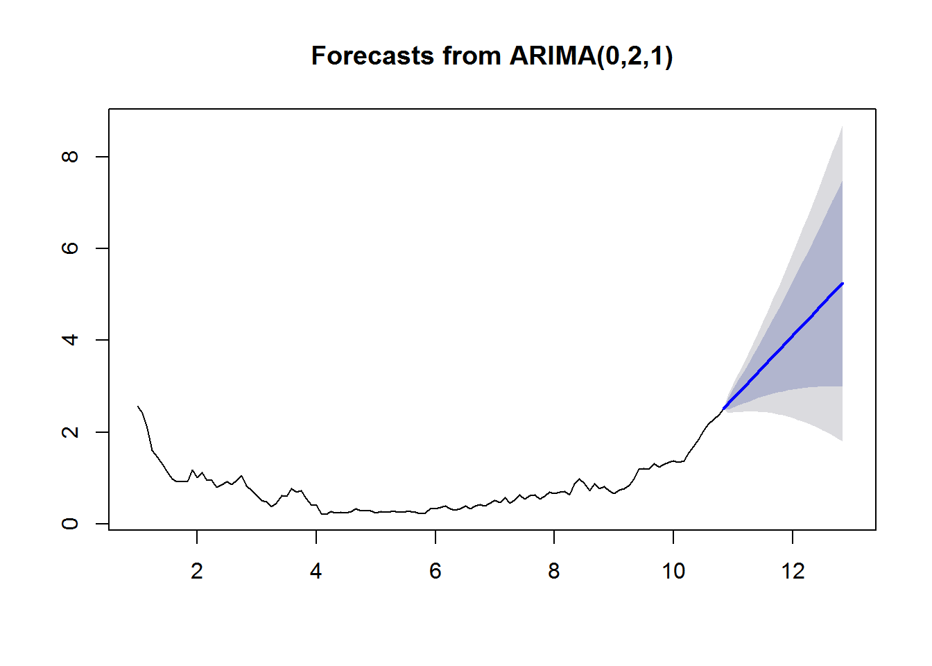
This is a simple effort at modeling 2-year treasury yields. It isn’t perfect, but it is a start. The initial work was to replicate this post. The author also kindly hosted this work on his github, which can be found here.
library(tidyquant)
library(forecast)
library(patchwork)
library(scales)


# pull data

monthly_twos <- tq_get("GS2",
                        get = "economic.data",
                        from = as.character(Sys.Date() - years(10)),
                        to   = as.character(Sys.Date()))

# plot

uc_ts_plot <- ggplot(monthly_twos, aes(date, price)) +
  geom_line(na.rm = TRUE) +
  geom_smooth(color = "green") +
  labs(x = "month",
       y = "yield") +
  scale_x_date(labels = date_format(format = "%b %Y"), breaks = date_breaks("1 year"))

uc_ts_plot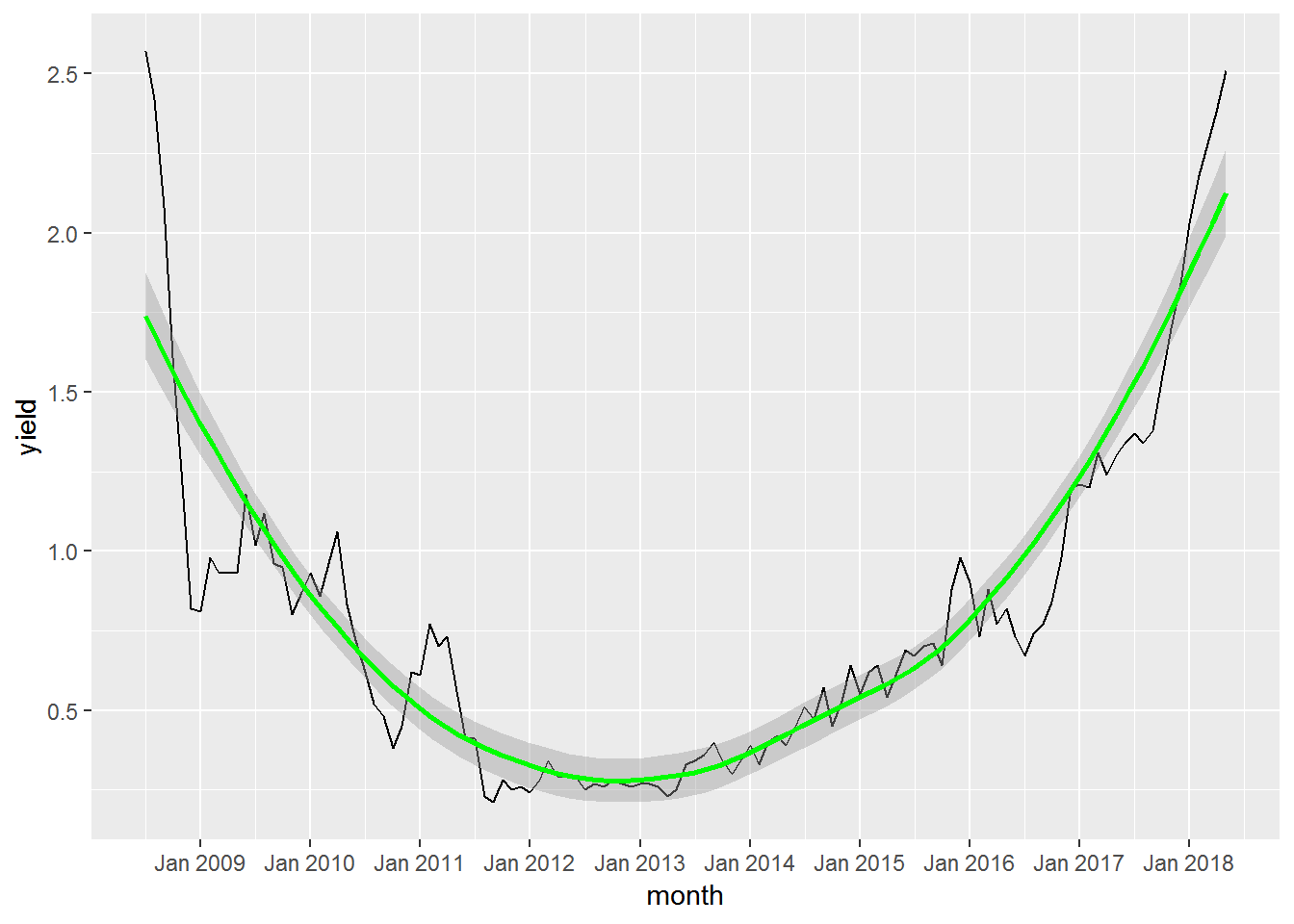
# create ts object and clean data

monthly_twos$ctwos <- tsclean(pull(monthly_twos[, "price"]))

c_ts_plot <- ggplot(monthly_twos, aes(date, ctwos)) +
  geom_line(na.rm = TRUE) +
  geom_smooth(color = "green") +
  labs(x = "month",
       y = "yield") +
  scale_x_date(labels = date_format(format = "%b %Y"), breaks = date_breaks("1 year"))

c_ts_plot + uc_ts_plot + plot_layout(ncol = 1)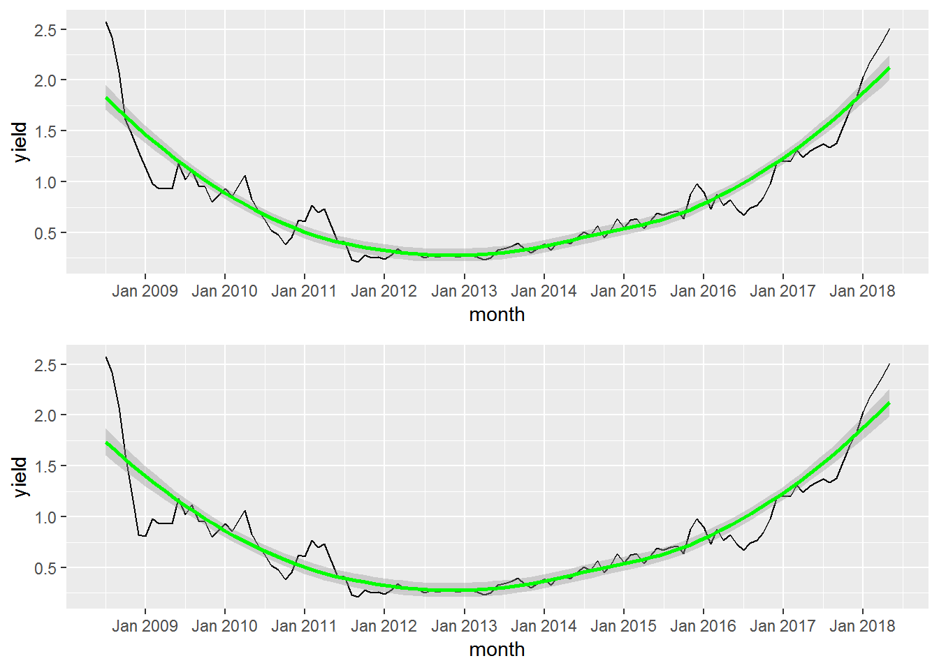
# change ts frequency and evaluate

my_ts <- ts(na.omit(monthly_twos$ctwos), frequency = 12)

plot(my_ts)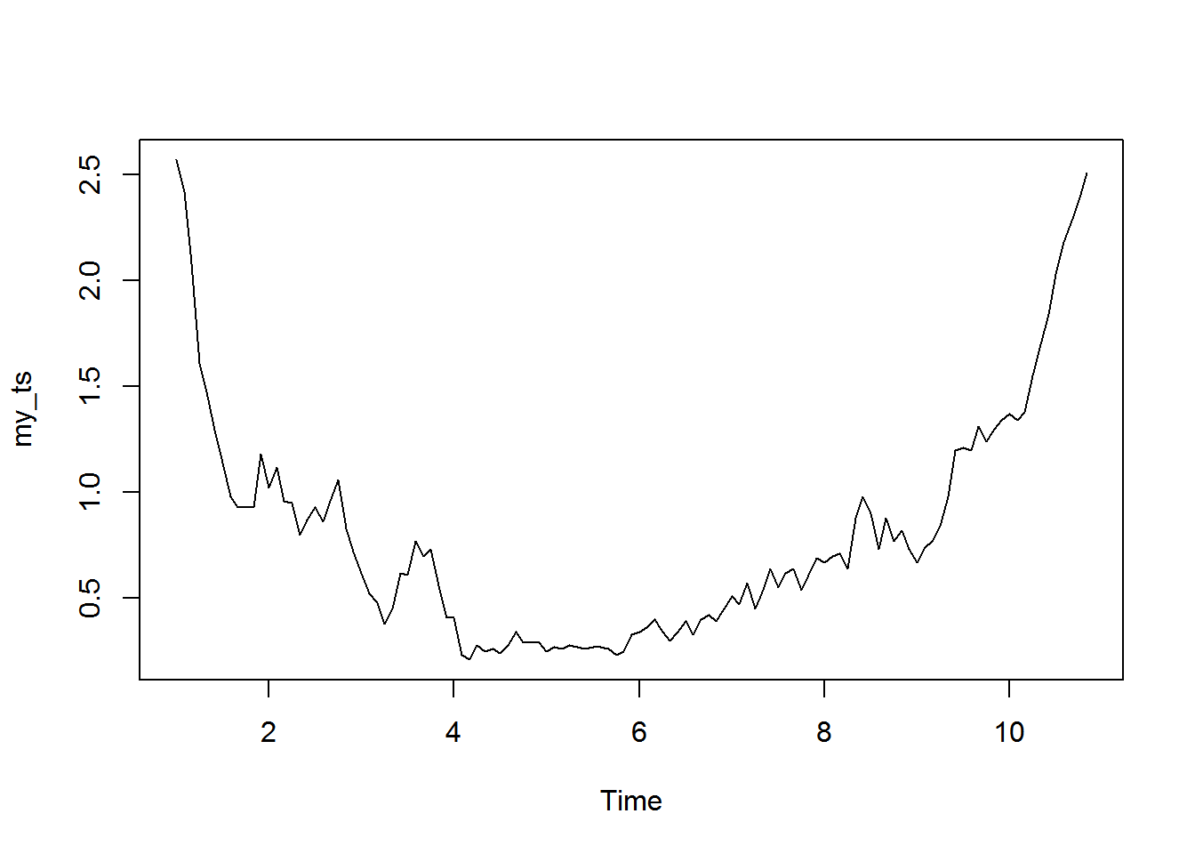
# run adf test to test for stationarity

tseries::adf.test(my_ts) # fail to reject null hypothesis that data series is stationary
##
## Augmented Dickey-Fuller Test
##
## data: my_ts
## Dickey-Fuller = 0.046027, Lag order = 4, p-value = 0.99
## alternative hypothesis: stationary# plot autocorrelation to determine order of differencing
Acf(my_ts) # shows autocorrelation at higher lags, we need to difference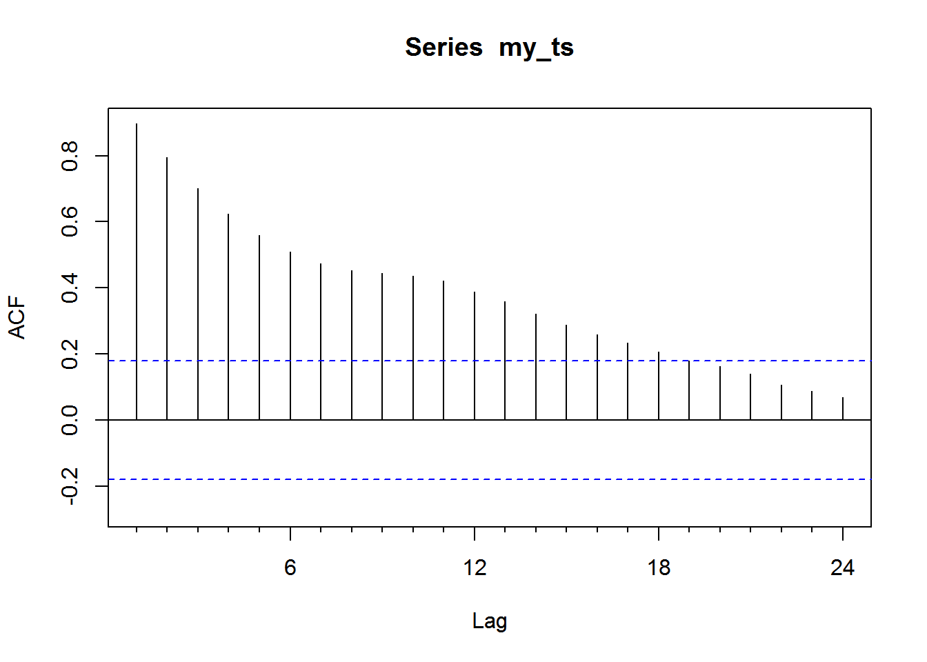
# fit first arima(0, 1, 0)(0, 0, 0) model

dfit1 <- arima(my_ts, order = c(0, 1, 0))

plot(residuals(dfit1))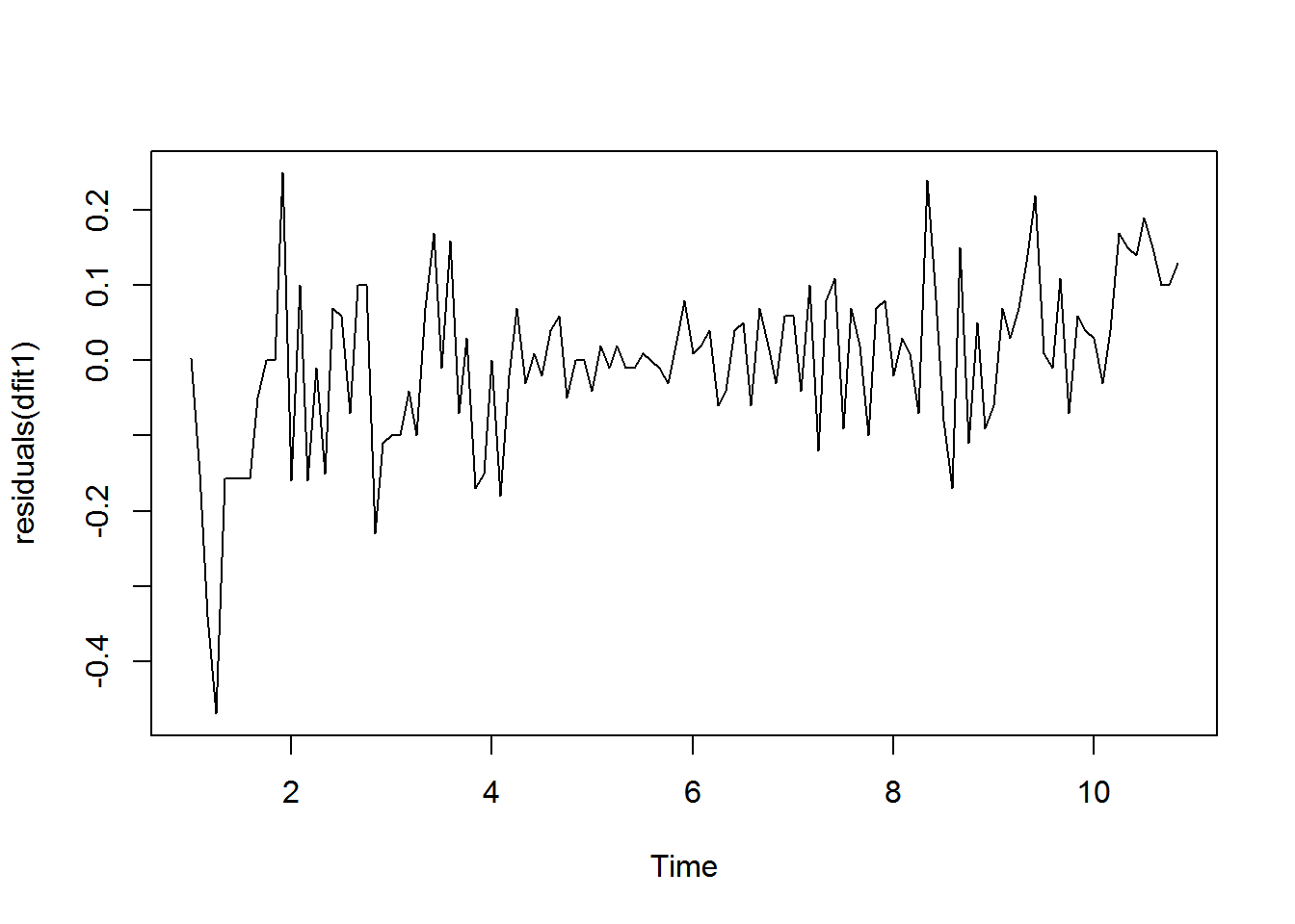
Acf(residuals(dfit1)) 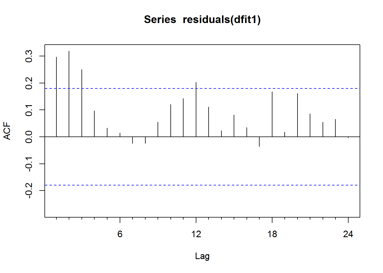
Pacf(residuals(dfit1))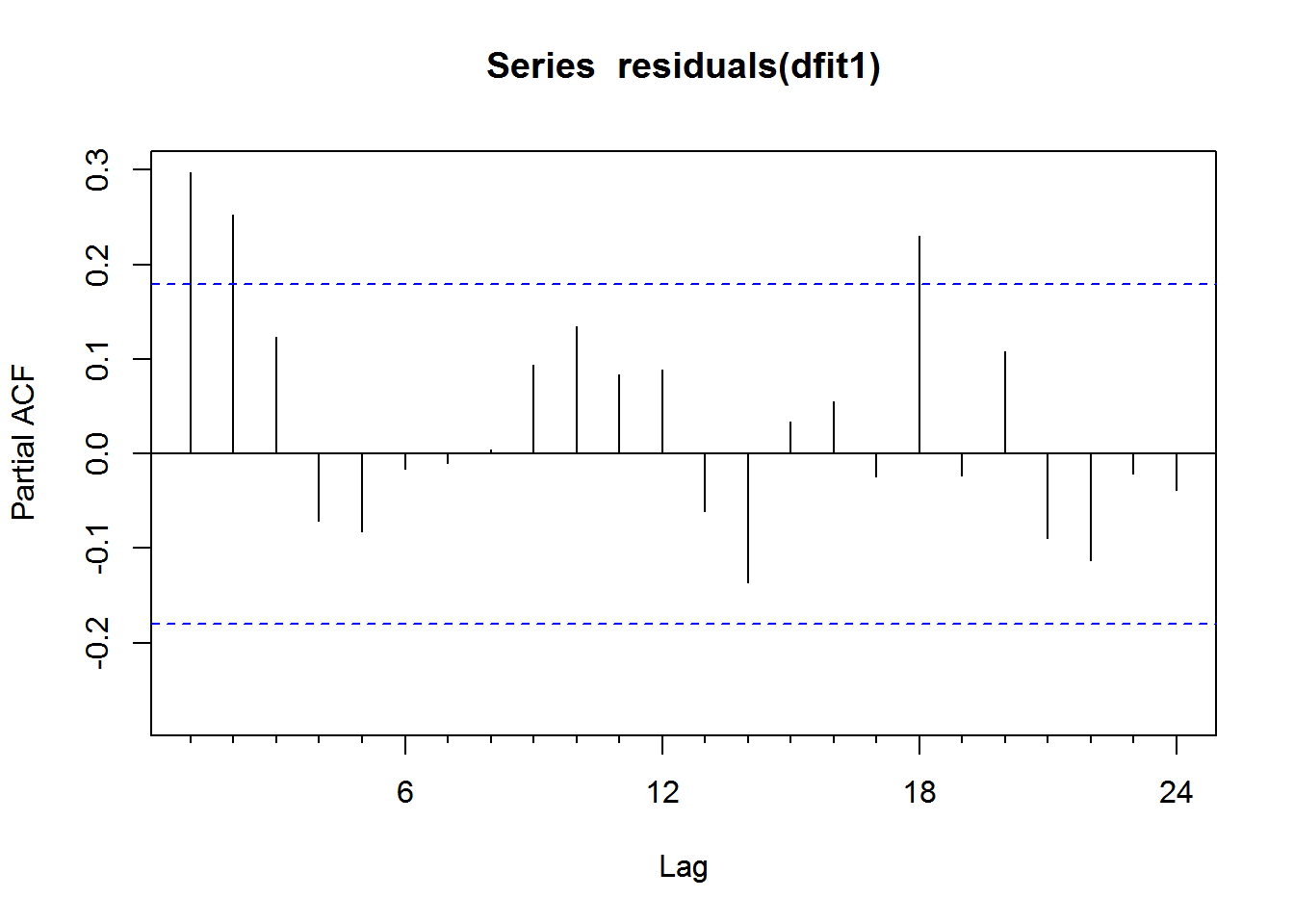
# identify ar/ma(p/q) and sar/sma(P/Q) components

dfit2 <- arima(my_ts, order = c(1, 1, 1))

plot(residuals(dfit2))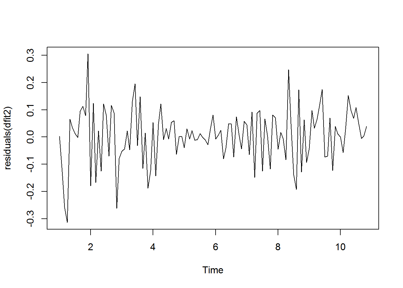
Acf(residuals(dfit2))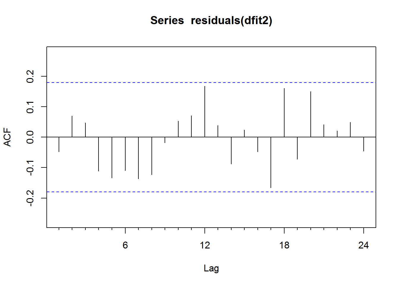
Pacf(residuals(dfit2))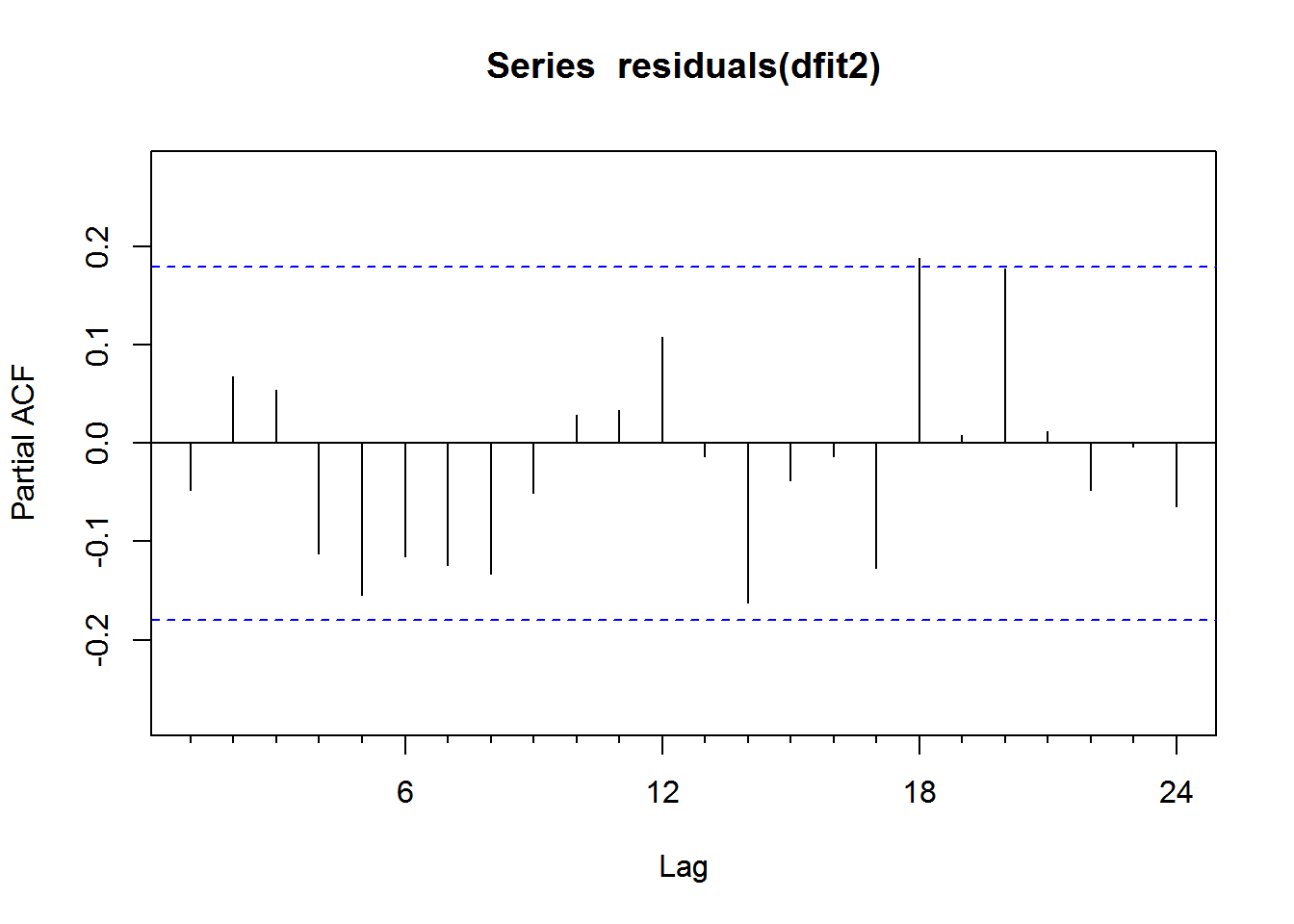
summary(dfit2)##
## Call:
## arima(x = my_ts, order = c(1, 1, 1))
##
## Coefficients:
## ar1 ma1
## 0.9302 -0.6992
## s.e. 0.1227 0.1995
##
## sigma^2 estimated as 0.01018: log likelihood = 102.91, aic = -199.82
##
## Training set error measures:
## ME RMSE MAE MPE MAPE MASE
## Training set 0.004713763 0.1004887 0.07646966 0.3012162 11.63798 0.9207571
## ACF1
## Training set -0.047908# check for statistical significance
lmtest::coeftest(dfit2)##
## z test of coefficients:
##
## Estimate Std. Error z value Pr(>|z|)
## ar1 0.93023 0.12267 7.5830 3.377e-14 ***
## ma1 -0.69916 0.19952 -3.5042 0.000458 ***
## ---
## Signif. codes: 0 '***' 0.001 '**' 0.01 '*' 0.05 '.' 0.1 ' ' 1# use auto.arima to see what model it generates
dfit3 <- auto.arima(my_ts, seasonal = FALSE)
plot(residuals(dfit3))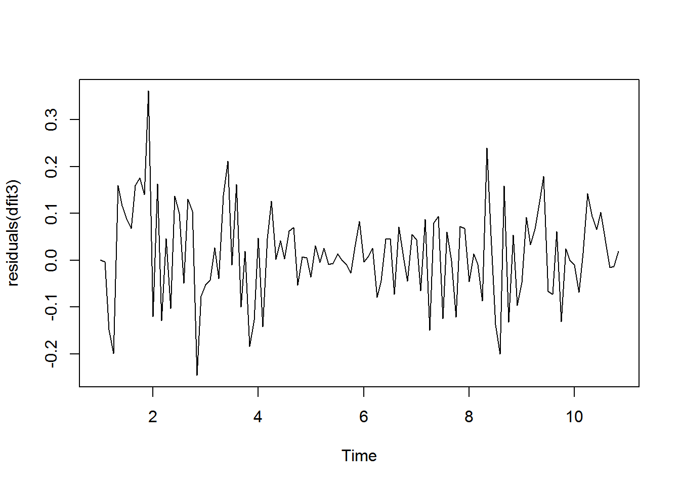
Acf(residuals(dfit3))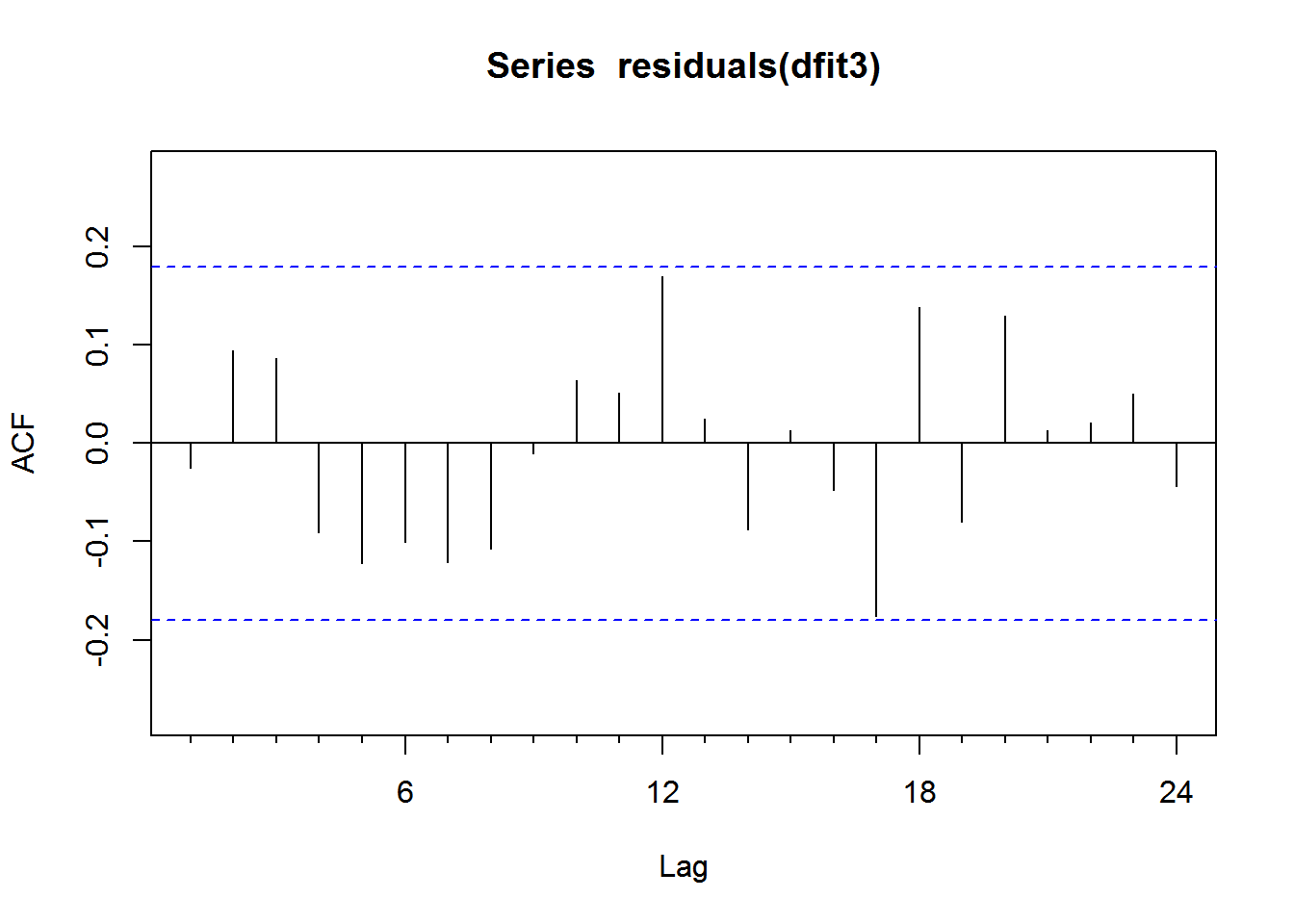
Pacf(residuals(dfit3))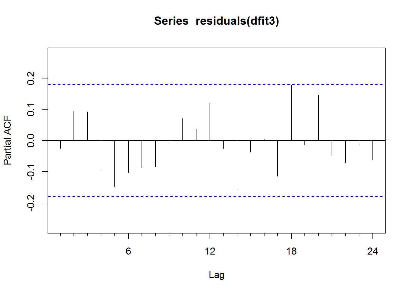
summary(dfit3)## Series: my_ts
## ARIMA(0,2,1)
##
## Coefficients:
## ma1
## -0.8030
## s.e. 0.0762
##
## sigma^2 estimated as 0.0103: log likelihood=101.62
## AIC=-199.24 AICc=-199.14 BIC=-193.72
##
## Training set error measures:
## ME RMSE MAE MPE MAPE MASE
## Training set 0.01432086 0.1002194 0.07744158 1.345159 11.82869 0.2459192
## ACF1
## Training set -0.0250633# auto.arima version actually outperforms
# model validation using n-fold holdout method
hold <- window(ts(my_ts), start = length(my_ts) - 11)
fit_predicted <- arima(ts(my_ts[-c((length(my_ts) - 11):length(my_ts))]),
order = c(0, 2, 2))
forecast_pred <- forecast(fit_predicted, h = 15)
plot(forecast_pred, main = "Predicted 2-Year Treasury Yield")
lines(ts(my_ts), col = "dark red")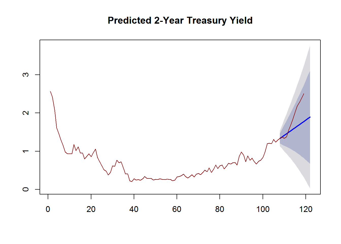
f_values <- forecast(dfit3, h = 24)

plot(f_values, showgap = FALSE)