Welcome to another edition of wrangling and plotting. Never one to bury the lede, today we cover rent versus buy trends across the U.S.A. Featuring prominently are the gtrendsR and geofacet packages. We use Google search volumes at the state level to understand housing market dynamics.
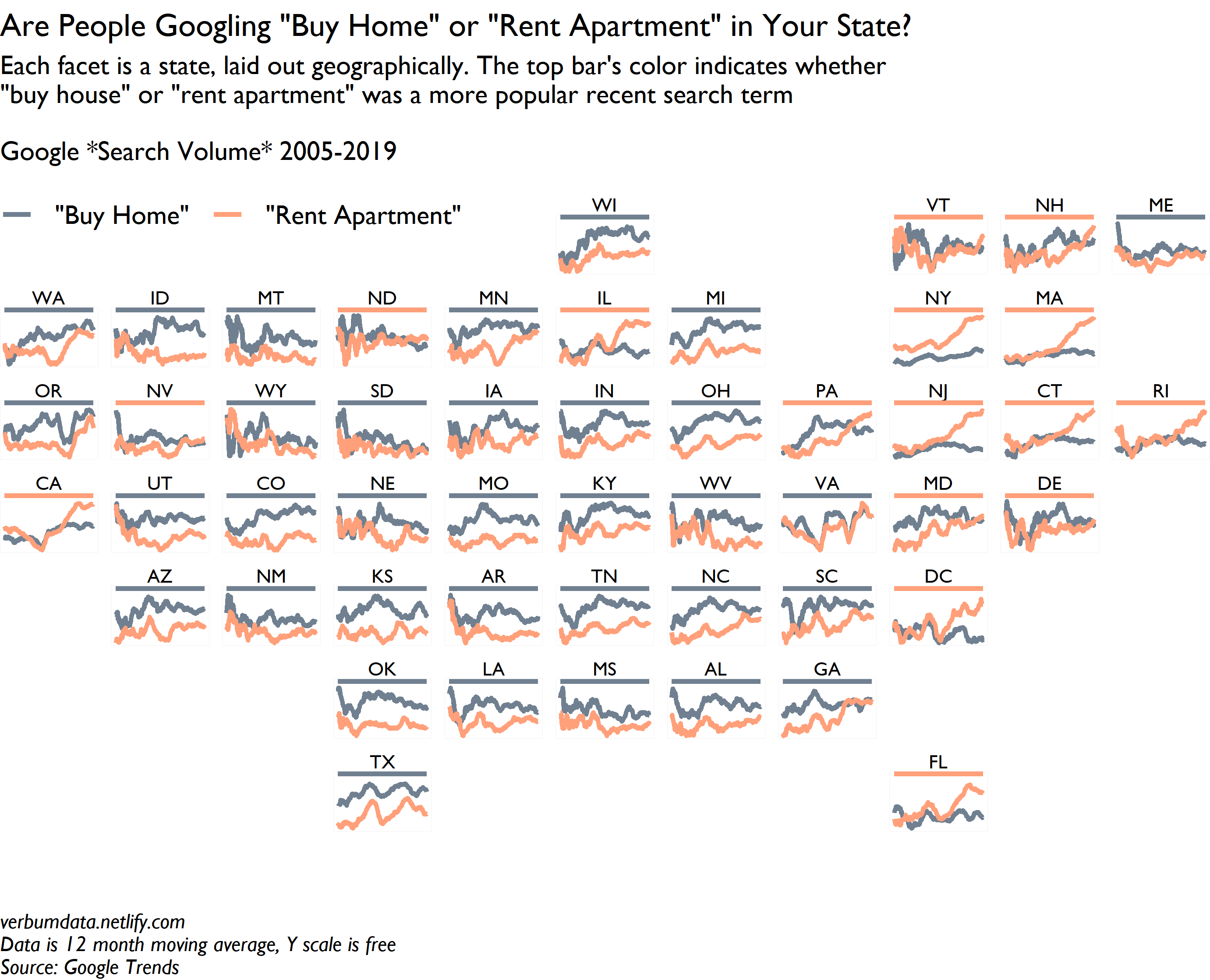
As usual, here is the plot towards which we work.

# load libraries

library(tidyverse)
library(gtrendsR)
library(lubridate)
library(zoo)
library(geofacet)
library(extrafont)
library(glue)
loadfonts(device = "win")
Get to ’ze data
The first thing to do is to import our county data. gtrendsR makes this easy enough. We just need to tinker a bit with the input data to get our desired region: the contiguous United States of America. Sorry HI & AK. To do that we attach the geography we want with some filters.
#attach data from gtrendsR package

data(countries)

# define lookup data

lookup <- countries %>%
  mutate_if(is.factor, as.character) %>%
  filter(country_code == "US") %>%
  filter(!sub_code %in% c("US-VI" ,"US-GU" ,"US-AS" ,
                          "US-PR", "US-UM", "US-MP")) %>%
  filter(str_length(sub_code) < 6 & str_length(sub_code) > 1) %>%
  distinct(sub_code) %>%
  pull()
Sweet and a touch scandalous. Now it’s onto accessing the Google Trends data. This isn’t an exact science. Results vary widely depending on one’s specific search term. I chose “buy home” and “rent apartment” as proxies for our home-interested and rent-interested populations. These two terms had similar search volume over our sample period at the national level. Once again, though, different search terms could produce different results.
# query google trends

gt_dat <- map(seq_along(lookup), ~ gtrends(c("buy home", "rent apartment"),
                                           geo = lookup[.x],
                                           time = "all")
              )

gt_interest <- map_df(gt_dat, ~ .x$interest_over_time) %>%
  mutate(month = month(date))
Bind n plot
Cool baby. Clean. Take a moment and reflect on the unbelievable parsimony of this call. We now possess state-level search trends for housing preference. Who said the 21st century isn’t the greatest of all time? Google (rightly) takes a lot of heat for privacy issues. We should at least be grateful Google exposes some of their treasure trove to users whose unwitting online activity makes it so sparkly and valuable.
Poetic waxing aside, I wasn’t always the biggest fan of geofaceting. However, reading this inspired post from the geofacet package creator Ryan Hafen convinced me it was the right approach to take with our Google search trend data.
### create the inital data frame for the plot

gt_plot <- gt_interest %>%
  select(date, keyword, hits, geo) %>%
  mutate(geo  = str_replace(geo, "US-", ""),
         year = year(date)) %>%
  group_by(keyword, geo) %>%
  mutate(year_ma_hits = rollmean(hits, 12, fill = NA, align = "right")) %>%
  filter(!is.na(year_ma_hits))
For the purposes of satisfying the sparse crowds visiting this page we subset our plot data frame into a few “keys.” These are aesthetic aids to make our plot the prettiest at the dance.
The first version of this plot lacked some of these touches. I doubt most readers will notice them at a first glance but I like to think they payoff as one studies the graphic.
Consider first the color-coded bars, made available in the val_key object. Deploying these segments above the plot enable us to quickly grasp the geographic distribution of rent vs. buy interest. Unsurprisingly, in states where land is more expensive (read, coastal areas and Chicagannoy [sic]) renting search volumes are ahead of ownership inquiries.
# recent search volume winner key

val_key <- gt_plot %>%
  group_by(geo, keyword) %>%
  filter(row_number() %in% c(n() - 1, n())) %>%
  summarize(avg = mean(year_ma_hits)) %>%
  spread(keyword, avg) %>%
  mutate(hi_val = ifelse(`buy home` > `rent apartment`, "home", "apt")) %>%
  filter(!geo %in% c("AK", "HI")) %>%
  split(., .$hi_val)

# vectorize me cap'n

apt_win <- val_key$apt$geo
home_win <- val_key$home$geo
Another item to clean up is the max value for each plot. With free y-axes, specifying the location of the colored segment described in the paragraph above was difficult. If one simply sets y = max(value) then one effectively locks all y-axes at the max search volume value across the entire dataset. By joining the max_val column we can refer to the local maximum for each state when faceting.
max_val <-  gt_plot %>%
  group_by(geo) %>%
  summarize(max = max(year_ma_hits)) %>%
  filter(!geo %in% c("AK", "HI"))

gt_plot_all <- gt_plot %>%
  left_join(max_val)
A final touch is the unorthodox subtitle/legend combination. I liked the positioning made available by this choice.
# create subtitle

cust_sub <- glue('
{str_wrap(\"Each facet is a state, laid out geographically. The top bar\'s color indicates whether \\"buy house\\" or \\"rent apartment\\" was a more popular recent search term\", 85)}

Google *Search Volume* 2005-2019

')
All said and done, we plot away.
# plot em up

ggplot(gt_plot_all, aes(date, year_ma_hits, color = keyword)) +
  geom_line(size = 1) +
  geom_segment(data = gt_plot_all %>% filter(geo %in% apt_win), # add apt bar
              aes(x = min(date), xend = max(date),
                  y = max * 1.1, yend = max * 1.1),
              color = "lightsalmon", size = 1) +
  geom_segment(data = gt_plot_all %>% filter(geo %in% home_win), # add buy bar
              aes(x = min(date), xend = max(date),
                  y = max * 1.1, yend = max * 1.1),
              color = "slategrey", size = 1) +
  scale_color_manual(labels = c('"Buy Home"', '"Rent Apartment"'),
                     values = c("slategrey", "lightsalmon")) +
  facet_geo(~ geo, grid = "us_state_contiguous_grid1", scales = "free_y") +
  theme_void(base_family = "Gill Sans MT") +
  guides(color = guide_legend(keywidth = unit(0.5, "cm"),
                              nrow = 1)) +
  theme(axis.text = element_blank(),
        axis.ticks = element_blank(),
        strip.text = element_text(size = 8),
        legend.position = c(0,1),
        legend.text = element_text(size = 11),
        legend.title = element_blank(),
        legend.spacing.x = unit(0.3, "cm"),
        legend.justification = "left",
        panel.border = element_rect(size = 0.1,
                                    color = "grey95",
                                    fill = NA),
        plot.caption = element_text(hjust = 0, face = "italic")) +
  labs(x = "",
       y = "",
       title = 'Are People Googling "Buy Home" or "Rent Apartment" in Your State?',
       subtitle = cust_sub,
       caption = "\n\n\nverbumdata.netlify.com\nData is 12 month moving average, Y scale is free\nSource: Google Trends")
The analytical consequences of the piece*
There is a lot of information to process in this chart. I offer the following observations:
New York provides a demonstration in both high land values and single-family home types. At no point since 2005 was “buy house” searched more than “rent apartment.” Part of this reflects the limited single-family supply in the state’s most populous city: NYC. Also, though, we can see the notable acceleration after the crisis as real estate values leaped higher on the back of a demand influx.
Nowhere in the Midwest is renting more searched than home buying, save Illinois. Chicago is the leading explanation for Illinois’s high rent search volume. The gap has narrowed in Kentucky, Iowa, and Tennessee. Minnesota rental interest has also closed in on purchase interest, but the relationship isn’t unprecedented. pre-financial crisis, many were as interested in renting as they were in buying.
Washington and Colorado, geographies of recent interest on this blog (specifically Seattle and Denver), offer different stories. Where homebuying and rental search volumes in Washington state have pushed higher across our sample, Colorado’s move is more muted. CO has seen relative search interest swing towards homeownership. Amazingly,
The outliers. Look at New England. Wow. Lots of rental interest. The Dakotas are bizarre, too. And home buying interest in Florida has never recovered from the Global Financial Crisis.