The Federal Open Market Committee (FOMC) released the minutes from its January 2019 meeting yesterday. For those searching for this fact’s relevance, your author conveys apologies, prayers, and understanding.
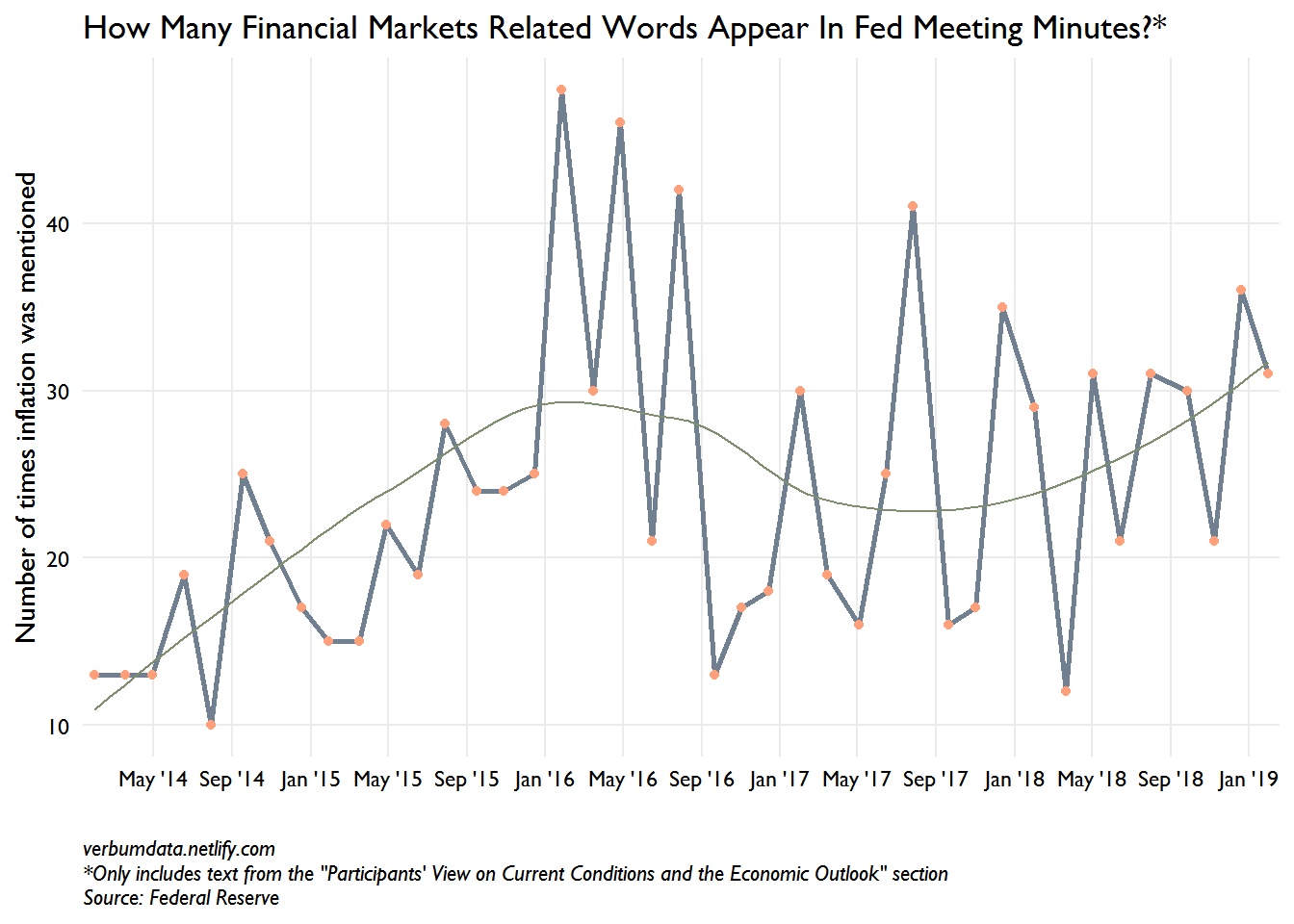
As always, here is our target output.

Scant are the meeting minutes that excite like the Fed’s. January’s meeting was especially unusual. In case you weren’t keeping score at home, the Fed made an about face in January, suggesting that instead of pursuing an aggressive interest rate hiking campaign until the fed funds rate was at 3%, they were content at current levels (2.25 - 2.50%).
Text mining was top of mind on the heels of this release. The main purpose of this post is to demonstrate a tidy, purrrful approach to webscraping. Please keep in mind that a search for https://www.federalreserve.gov/robots.txt produced a 404 page not found error. We are thus good to fire at will!
A word of caution: the large character vectors in this exercise take a long time to print in console, especially on slow machines.
The basics & the links
# import packages, fonts, and set a theme

library(tidyverse)
library(rvest)
library(tidytext)
library(lubridate)
library(extrafont)
loadfonts(device = "win")

theme_set(theme_minimal() +
            theme(text = element_text(family = "Gill Sans MT", colour = "black")))
We want to look at historical meeting minutes. In some respects, the Fed’s website is a scrapers dream. One page contains the entire history of all the links we could ever want. Load up the base page, pull off all the links, and find those which contain “minutes” and “some digits” and voila.
# read base page

base_pg <- read_html("https://www.federalreserve.gov/monetarypolicy/fomccalendars.htm")

# extract minutes links

min_links <- base_pg %>%
  html_nodes("#article") %>% # narrow down the scrape space
  html_nodes("a") %>% # call this to access href
  html_attr("href") %>%
  .[grepl("minutes\\d+.htm", .)] %>% # see note above
  paste0("https://www.federalreserve.gov", .) # create real links
Purrring our way towards minutes
Links are built. Now we read in the pages. This takes a moment. You should save down an .rds of the scraped data so as not to tax the poor .gov server.
The last processing step to go full tidy is to create a tibble with the date from each meeting (extracted from the links), the minutes text, and then a subset of the minutes text which is most interesting.
Those curious about why I selected the Participants’ Views on Current Conditions and the Economic Outlook section would do well to peruse the actual meeting minutes. For our purposes, the smaller selection sharpens the signal/noise ratio.
# retrieve minutes text

fomc_min <- map(min_links, ~
                  read_html(.x) %>%
                  html_nodes("p") %>%
                  html_text()
    )

# good scraping hygiene would have you saveRDS(fomc_min, "c:/users/your_desired/directory.rds")
# for later use and/or analysis
This puppy might want a bit of explaining. The key items are the gsub, which kills the newline and carriage return characters, the paste which concatenates all our little p html nodes’ text, and the final regex which subsets text of interest.
# combine into dataframe

fomc_df <- tibble(
  date = str_extract(min_links, "\\d+"),
  min_text = map_chr(fomc_min, ~ paste(gsub("[\n\r]" , " ", .x), collapse = "")),
  part_view = str_extract(min_text, "(?<=Current Conditions and the Economic Outlook).*(?=Committee Policy Action)")
) %>%
  mutate_at(vars(min_text, part_view), funs(str_remove_all(., "\\d{1,}[\\,\\.]{1}\\d{1,}|\\d+")))
Time to tidy text
Onto the tidiest of texting Fed minutes edition. We follow an established workflow here. Our main interest will be in finding the change in words like “financial”, “market participants”, “financial markets”, etc. My bet (stated before I’ve made the chart) is that we see a run-up in January and last December. I’d also bet that you’ll see a spike in August and September of 2015, right after the Chinese devaluation, when the Fed punted on hiking until December. I’ve got a little hack for the bigrams…
# unnest tokens

tok_part <- fomc_df %>%
  select(-min_text) %>%
  mutate(date = ymd(date)) %>%
  unnest_tokens(word, part_view) %>%
  anti_join(stop_words)

# words of interest

fin_words <- paste("financial", "yield", "equity", "bond",
                   "loan", "credit", "stocks", "dollar",
                   "oil", "asset", "curve", "commodity",
                   sep = "|")
We’ve got our tokenized data. Now lets find and plot our words. As mentioned, we will have to do a little hack to get the 2 word pairs.
# plot

fin_cond <- tok_part %>%
  mutate(fin_word = if_else(str_detect(word, fin_words), 1, 0),
         fin_bi = case_when(
           str_detect(word, "financial") & str_detect(lead(word, 1), "market|condition") ~ 1,
           str_detect(word, "equity|stock") & str_detect(lead(word, 1), "price") ~ 1,
           str_detect(word, "market") & str_detect(lead(word, 1), "participants") ~ 1,
           str_detect(word, "money") & str_detect(lead(word, 1), "market") ~ 1,
           TRUE ~ 0),
         fin_fin = if_else(fin_word == 1 | fin_bi == 1, 1, 0)
         )

fin_cond %>%
  group_by(date) %>%
  summarize(fin_word = sum(fin_fin)) %>%
  ggplot(aes(date, fin_word)) +
  geom_line(color = "slategrey", size = 1) +
  geom_point(color = "lightsalmon") +
  geom_smooth(se = FALSE, color = "#7f8e6f", size = 0.5) +
  scale_x_date(date_breaks = "4 months", date_labels = "%b '%y",expand = c(0.01,.01)) +
  labs(x = "",
       y = "Number of times inflation was mentioned",
       title = 'How Many Financial Markets Related Words Appear In Fed Meeting Minutes?*',
       caption = 'verbumdata.netlify.com\n*Only includes text from the "Participants\' View on Current Conditions and the Economic Outlook" section\nSource: Federal Reserve') +
  theme(panel.grid.minor = element_blank(),
        axis.text = element_text(color = "black"),
        plot.caption = element_text(face = "italic", hjust = 0))
Well folks, you author isn’t perfect. The predicted spike in late 2015 really appeared in early 2016 (when oil prices hit $27 a barrel). There is a notable spike at the December 2018 meeting, as well.
The data is rather noisy but the trend line is quite clear. Financial market concerns are on the rise at the Fed. We are quite keen to track this into the future.