Rejoice readers! The dearly beloved GLORIA St. Louis Blues made the Stanley Cups finals after a convincing drubbing of the San Jose Sharts. You will no doubt recall the hockey team abbreviated STL is the oldest active NHL team to never have won a Stanley Cup.
The purpose of our next few posts is to examine the common narrative about the Blues that they went from being the NHL’s worst team in the 1st half of the year to being the NHL’s best team in the 2nd half of the year. Here are the steps we will take to do so, with the help of our indomitable friend R.
Today, on the day of the first Stanley Cup game, we will do two things.
- Pull all game data for each team for the 2018-2019 season
- Establish basic performance facts
And, as usual, here is the moneymaker chart from the day’s proceedings.

library(tidyverse)
library(rvest)
library(lubridate)
library(zoo)
extrafont::loadfonts(device = "win")

theme_set(theme_minimal(base_family = "Gill Sans MT"))

blues_colors <- c("#002e88", "#ffc72b", "#304767")
Pulling the game data
The lovely hockey-reference.com features all our required information. Let us pull.
# retrieve three digit codes for each team

link <- read_html("https://www.hockey-reference.com/leagues/NHL_2019_standings.html")

# select the standings table and pull the underlying links

full_names <- link %>%
  html_node(xpath = '//*[@id="standings"]') %>%
  html_table() %>%
  .[, 2]

three_letters <- link %>%
  html_node(xpath = '//*[@id="standings"]') %>%
  html_nodes("a") %>%
  html_attr("href") %>%
  gsub("[^A-Z]", "", .)

team_name_df <- tibble(abbr = three_letters,
                       team = full_names)

# build our link list

link_list <- paste0('https://www.hockey-reference.com/teams/', team_name_df$abbr, '/2019_gamelog.html')

# pull data

season_stats <- map_df(seq_along(link_list), ~ {

       stats <- read_html(link_list[.x]) %>%
         html_nodes("table") %>%
         html_table(header = FALSE) %>%
         bind_rows(.id = "epoch")

       stats <- stats[, colSums(!is.na(stats)) != 0]

       names(stats) <- c(
         "epoch", "gp", "date", "h_a", "opponent", "gf", "ga",
         "result", "ot", "t_s", "t_pim", "t_ppg", "t_ppo", "t_shg",
         "o_s", "o_pim", "o_ppg", "o_ppo", "o_shg", "a_cf", "a_ca",
         "a_cf_pct", "a_ff", "a_fa", "a_ff_pct", "a_fow", "a_fol",
         "a_fo_pct", "a_ozs_pct", "a_pdo"
       )

       stats <- as_tibble(stats[-c(1:2), ]) %>%
         filter(!grepl("Opponent", opponent), nchar(opponent) != 0) %>%
         mutate(team = tolower(team_name_df$team[.x]),
                opponent = tolower(opponent),
                gp = as.numeric(gp),
                h_a = ifelse(nchar(h_a) == 0, "home", "away"),
                result = ifelse(result == "L", 0, 1),
                ot = case_when(
                  ot == "OT" ~ "ot",
                  ot == "SO" ~ "so",
                  TRUE ~ "reg"
                  ),
                epoch = case_when(
                  epoch == 1 ~ "rs",
                  epoch == 2 ~ "playoff"
                  ),
                points = case_when(
                  epoch == "rs" & result == 1 ~ 2,
                  epoch == "rs" & result == 0 & ot %in% c("ot", "so") ~ 1,
                  TRUE ~ 0),
                points_total = cumsum(points)
                ) %>%
         select(epoch:h_a, team, opponent, result, ot, points_total, gf:a_pdo) %>%
         mutate_at(vars(gf:a_pdo), list(as.numeric))
       }
       )
With all the data pulled let’s check to make sure it is accurate.
season_stats %>%
  group_by(team) %>%
  summarize(pts = max(points_total)) %>%
  arrange(-pts)
## # A tibble: 31 x 2
## team pts
## <chr> <dbl>
## 1 tampa bay lightning 128
## 2 boston bruins 107
## 3 calgary flames 107
## 4 washington capitals 104
## 5 new york islanders 103
## 6 san jose sharks 101
## 7 nashville predators 100
## 8 pittsburgh penguins 100
## 9 toronto maple leafs 100
## 10 carolina hurricanes 99
## # ... with 21 more rowsEstablishing basic performance facts
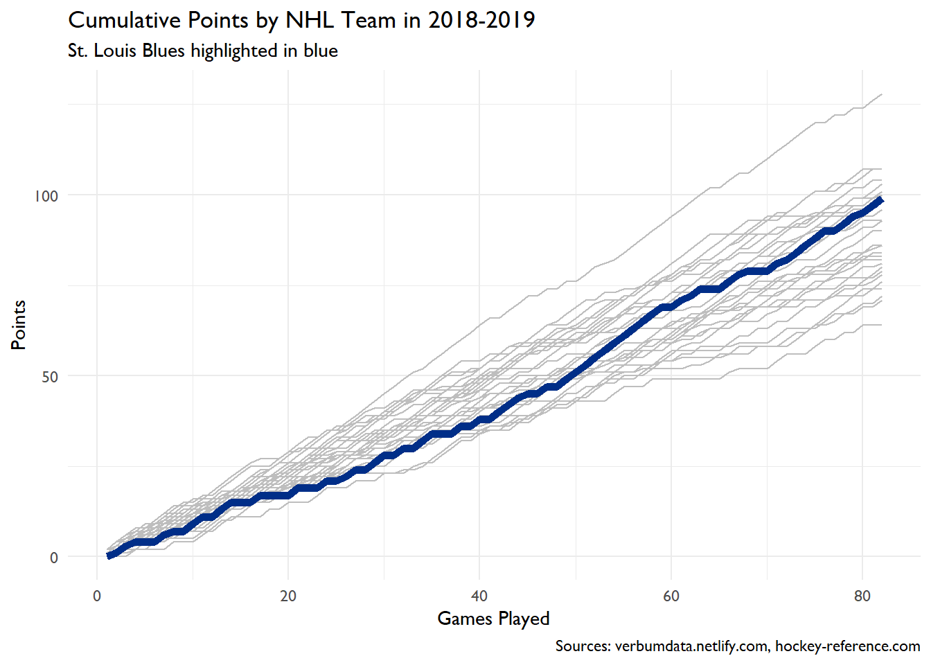
Now for fun, let’s plot each team’s cumulative points over the season.
reg_season <- season_stats %>% filter(epoch == "rs")

ggplot() +
  geom_line(data = reg_season %>% filter(!team %in% "st. louis blues"),
       aes(gp, points_total, group = team),
       color = "grey") +
  geom_line(data = reg_season %>% filter(team %in% "st. louis blues"),
       aes(gp, points_total, group = team),
       color = blues_colors[1],
       size = 2) +
  labs(x = "Games Played",
       y = "Points",
       title = "Cumulative Points by NHL Team in 2018-2019",
       subtitle = "St. Louis Blues highlighted in blue",
       caption = "Sources: verbumdata.netlify.com, hockey-reference.com")
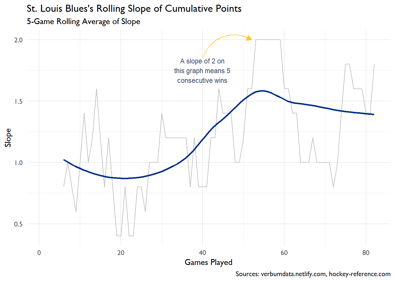
Just after the 50th game, the Blues really accelerated. But we can put a finer grain on the Blues’s acceleration. Let’s look at the rolling 5 game slope of performance. The Blues won 11 consecutive games from 2019-01-23 to 2019-02-19! That is quite a run.
reg_season %>%
  filter(team %in% "st. louis blues") %>%
  mutate(slope = points_total - lag(points_total, 1),
         roll_slope = rollmean(slope, 5, na.pad = TRUE, align = "right")
  ) %>%
  ggplot(aes(gp, roll_slope)) +
  geom_line(color = "grey") +
  geom_smooth(method = "loess", se = FALSE, color = blues_colors[1]) +
  geom_curve(data = reg_season %>% filter(team %in% "st. louis blues"),
             aes(x = 40, xend = 52,
                 y = 1.85, yend = 2),
             color = blues_colors[2],
             curvature = -0.5,
             arrow = arrow(length = unit(0.25, "cm"),
                           type = "closed")) +
  annotate("text", x = 40, y = 1.75,
           label = str_wrap("A slope of 2 on this graph means 5 consecutive wins", 20),
           size = 3,
           color = blues_colors[3],
           hjust = 0.5) +
  labs(x = "Games Played",
       y = "Slope",
       title = "St. Louis Blues's Rolling Slope of Cumulative Points",
       subtitle = "5-Game Rolling Average of Slope",
       caption = "Sources: verbumdata.netlify.com, hockey-reference.com")
## Warning: Removed 5 rows containing non-finite values (stat_smooth).## Warning: Removed 5 rows containing missing values (geom_path).
We’ve established basic performance facts. We know that the Blues dramatically accelerated their play over the first few months of 2019. Over the course of the Stanley Cup Finals, we will dive into the reasons behind their elevation. The next tasks are as follows:
- Look at the Blues’s dynamics over the season
- Compare changes witnessed in STL with other teams in the league
Thank you all for reading.