Vice Plotted

Getting the data

Bless the internet. A few minutes of searching brought to my solid state memory a Vice script. I cannot positively affirm its accuracy, but a cursory glance satisfied my concerns. Here’s the import process.

# load libraries

library(pdftools)
library(tidytext)
library(tidyverse)
library(extrafont)
loadfonts(device = 'win')

# read in the text of the script

text <- pdf_text('https://s3-us-west-2.amazonaws.com/script-pdf/vice-script-pdf.pdf')

We interrupt your programming with a note on programming

Now, before proceeding to the text processing, please forgive a minor digression.

A chief point of recent programming musing has been the utility of deploying only base R in my analyses. Experiences with other R script users at work are the cause of these musings. Avoiding dependencies makes life much easier in production settings with novice R colleagues.

You will see the results of my attitude in the code below. If only as an exercise, I have begun to write as much of my data processing scripts in base R. Some of the solutions may be ungainly but they are sure to work in 10 years. For readers of the NHL Poisson modeling post wondering why data.table features prominently, the answer lies in a similar attempt to practice with a more minimalist code base.

Text processing begins

With the script located we turn now to text processing. The pdftools package is terrific. Making the most of it, though, usually requires heavy regex. The first pass removes new lines and returns and adjusts George W Bush’s name to make later processing easier.

# clean up the text of the script

text_clean <- gsub("[\\\r\\\n]|\\(.+?\\)", " ", text, perl = T)

text_clean <- gsub('W BUSH', 'WBUSH', text_clean)

The modestly clean text belongs in a data.frame.

# create data frame with page number

vice_df <- data.frame(text = gsub('\\s+', ' ', text_clean), stringsAsFactors = FALSE, row.names = NULL)

vice_df$pg <- as.numeric(row(vice_df))

My main interest in this short analysis is with Lynne and Dick Cheney. To conduct the study we will need to separate out their lines and put them into a clean format in the data.frame. The for loop is not ideal, but in the base R idiom, it made life easier than negotiating an apply beast into a character vector.

The regex extraction code also shows why we ought to be thankful for CRAN and libraries. What could be done simply and easily with stringr::str_extract_all instead requires a full trimws(regmatches(text, regexpr(regex, text))) adventure. At least it will be stable!

# extract lynne's lines into new column, first initialize

vice_df$lynne_lines <- NA

for(i in seq_along(vice_df$text)) {
  
  # check if lynne speaks on the page
  
  if(grepl('(?<=LYNNE).+?(?=\\w+[A-Z]\\b)', vice_df$text[i], perl = T)) {
    
    # if she does, extract from LYNNE until the next ALL CAPS word
    
    vice_df$lynne_lines[i] <- trimws(regmatches(vice_df$text[i], 
                                         regexpr('(?<=LYNNE).+?(?=\\w+[A-Z]\\b)', vice_df$text[i], perl = T))
    )
  }
}

# now get dicks lines

vice_df$dick_lines <- NA

for(i in seq_along(vice_df$text)) {
  
  # check if lynne speaks on the page
  
  if(grepl('(?<=DICK).+?(?=\\w+[A-Z]\\b)', vice_df$text[i], perl = T)) {
    
    # if she does, extract from LYNNE until the next ALL CAPS word
    
    vice_df$dick_lines[i] <- trimws(regmatches(vice_df$text[i], 
                                         regexpr('(?<=DICK).+?(?=\\w+[A-Z]\\b)', vice_df$text[i], perl = T))
    )
  }
}

The last of the cleaning deals with funky text processing residuals: removing short, nonsensical “words”, setting all text tolower and removing page number concatenations.

# clean up final df

rid_shorty <- function(text, nchar = 2 ) {
  ifelse(nchar(text) <= nchar, NA_character_, text)
}

# apply function

vice_df[,c("lynne_lines", "dick_lines")] <- sapply(vice_df[,c("lynne_lines", "dick_lines")], rid_shorty)

# turn all char cols to lower

vice_df[, !names(vice_df) %in% "pg"] <- lapply(vice_df[, !names(vice_df) %in% "pg"], tolower)

# final cleaning

vice_df$text <- gsub('^\\s+[0-9].+?(?=\\w)', '', vice_df$text, perl = TRUE)

Eyes turn to analyze!

Our first task will be to categorize and count Lynne and Dick’s words by emotion. Regular readers are sure to expect the handy tidytext package. And indeed their expectations are correct. We will use the NRC word-emotion association lexicon to help us in our quest.

# text analysis

vice_tidy <- as_tibble(vice_df) %>% 
  gather(character, line, lynne_lines:dick_lines) %>% 
  mutate(character = gsub('_.+$', '', character))

# characters only

character_lines <- vice_tidy[!is.na(vice_tidy$line), !names(vice_tidy) %in% "text"] %>% 
  unnest_tokens(word, line) %>% 
  anti_join(stop_words) %>% 
  inner_join(get_sentiments("nrc")) %>% 
  count(character, sentiment) %>% 
  group_by(character) %>% 
  arrange(-n, .by_group = TRUE) %>% 
  ungroup() %>% 
  mutate(sent_rank = paste0(row_number(), '_', sentiment),
         character = str_to_title(character))

# now we plot

ggplot(character_lines, aes(fct_reorder(sent_rank, n), n, fill = sent_rank)) +
  geom_col() +
  scale_fill_viridis_d() +
  coord_flip() +
  guides(fill = FALSE) +
  facet_wrap(~ character, scales = "free") +
  scale_x_discrete(labels = function(x) str_to_title(gsub('\\d+_', '', x)), expand = c(0,0)) +
  scale_y_continuous(expand = c(0,0)) +
  expand_limits(0,0,0,0) +
  theme_minimal(base_family = 'Gill Sans MT') +
  labs(x = '',
       y = 'Word Count',
       title = "Sentiment Analysis of *Vice* Main Characters' Lines",
       caption = 'Source: verbumdata.netlify.com') +
  theme(strip.text = element_text(color = 'black', face = 'bold', size = 11),
        axis.ticks = element_blank(),
        axis.text = element_text(color = 'black'),
        axis.line = element_line(color = 'black'),
        panel.grid.minor = element_blank(),
        plot.caption = element_text(hjust = 0, face = 'italic', family = 'serif'))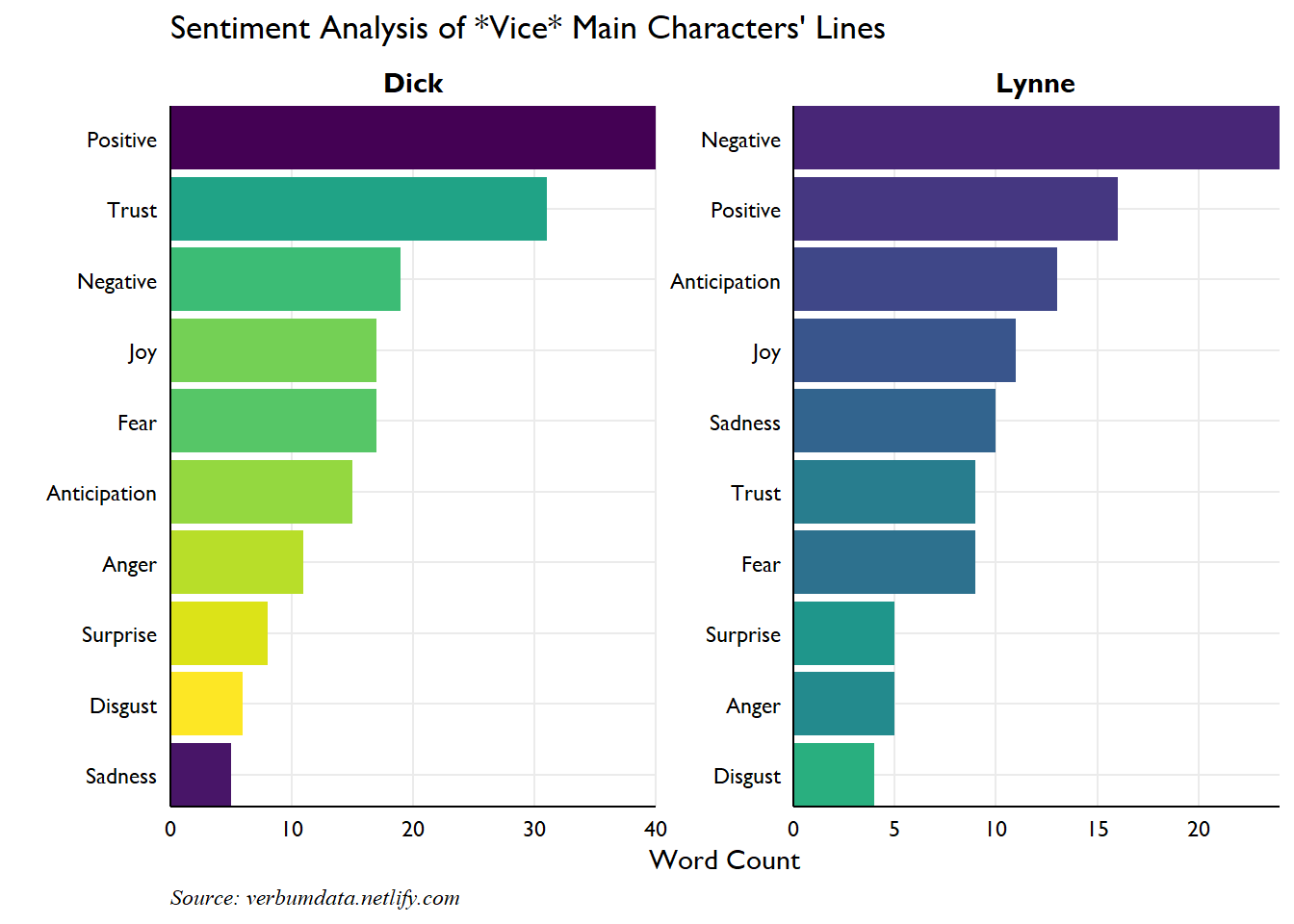

I don’t know about you but I was surprised to find just how positive Dick’s lines are in the movie. Say what you will about Adam McKay’s politics, but one would be hard pressed to accuse him of undue negative characterization of Dick Cheney.

Lynne, on the other hand, is considerably more negative. She leaks anger and frustration throughout. Part of the pessimism is her own struggle to define personal meaning in her maternal role. But the evidence also supports an underlying trouble which never disappears despite her personal advancement. She can never find contentment and pushes her husband relentlessly throughout.

SPOILER ALERT The final scenes of the flick show Lynne sacrificing her relationship with one daughter to elevate the political prospects of her other daughter. This vindictive choice is one never made by Dick, at least not in the movie. He privileges his offspring equally, no matter their life choices.

Pulling it all together

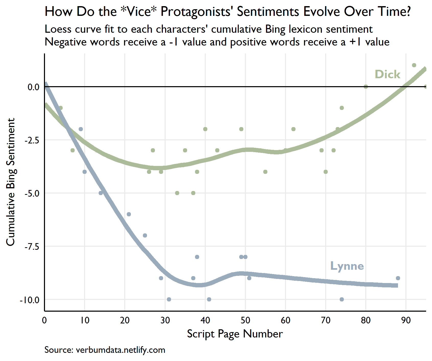
The static look at Dick and Lynne’s word choices compelled deeper questions. I immediately began to wonder how the pair’s sentiment evolves over the course of the movie. My finding shocked my eyes. Alas, the closer, begins here.

# create cumulative sentiment for each character

sentiment_time <- vice_tidy[!is.na(vice_tidy$line), !names(vice_tidy) %in% "text"] %>% 
  unnest_tokens(word, line) %>% 
  anti_join(stop_words) %>% 
  inner_join(get_sentiments("bing")) %>% 
  filter(word != "dick") %>% 
  mutate(sent_val = ifelse(sentiment == "negative", -1, 1)) %>% 
  group_by(pg, character) %>% 
  summarize(sent = sum(sent_val)) %>% 
  group_by(character) %>% 
  mutate(cum_sent = cumsum(sent))

# initialize each character at zero

initial_condition <- tibble(
  pg = c(0, 0),
  character = c("lynne", "dick"),
  sent = c(0, 0),
  cum_sent = c(0, 0)
)

# bind each

cum_sent_data <- bind_rows(initial_condition, sentiment_time)

We have our data locked and loaded. The methodology used here is as follows. For each character, words matched with “positive” or “negative” sentiment in the Bing database receive either a +1 or a -1 score. With the scoring done, we take a cumulative sum for each character over the life of the script to evaluate the level and evolution of their respective sentiments.

# plot

ggplot(cum_sent_data, aes(pg, cum_sent, color = character)) +
  geom_point(show.legend = FALSE) +
  geom_smooth(method = "loess", se = FALSE, size = 2, show.legend = FALSE) +
  geom_text(data = cum_sent_data %>% group_by(character) %>% filter(pg == max(pg)),
            aes(pg, cum_sent, color = character, label = tools::toTitleCase(character)),
            hjust = 2,
            vjust = -1,
            show.legend = FALSE,
            family = "Gill Sans MT",
            fontface = "bold",
            size = 4) +
  geom_hline(yintercept = 0) +
  scale_color_manual(values = c("#acbc9a", "#9aacbc")) +
  scale_x_continuous(breaks = seq(0, max(cum_sent_data$pg), 10), expand = c(0, 0)) +
  theme_minimal(base_family = 'Gill Sans MT') +
  labs(x = 'Script Page Number',
       y = 'Cumulative Bing Sentiment',
       title = "How Do the *Vice* Protagonists' Sentiments Evolve Over Time?",
       subtitle = "Loess curve fit to each characters' cumulative Bing lexicon sentiment\nNegative words receive a -1 value and positive words receive a +1 value",
       caption = 'Source: verbumdata.netlify.com') +
  theme(axis.text = element_text(color = 'black'),
        axis.line = element_line(color = 'black'),
        plot.caption = element_text(hjust = 0),
        panel.grid.minor = element_blank(),
        legend.position = "top",
        legend.title = element_blank())

What a plot! Many items deserve noting.

First, the clear difference in sentiment observed in our first plot plays out completely here. While the overall tone of matched words tends to be negative for both characters throughout the movie, Dick is cumulatively more positive than Lynne at nearly every point.

Second, Lynne is monstrously negative throughout the entire movie. She descends to her sentimental nadir 1/3 of the way into the movie and never recovers. This period corresponds to Dick’s early arrival in Washington as he fights to find his way. Dick’s cumulative sentiment drops through the first 1/3 of the movie, too, but not nearly as sharply.

Third, Dick recovers and Lynne does not. As soon as Dick’s cumulative nadir occurs right around the time he is made the youngest Chief of Staff in history (page 31). From there, his trajectory is up. His political career (and later commercial career) finds its footing and he turns more positive as he accrues power.

The final item worthy of note is the sharp drop in matched Lynne sentiment through the last half of the movie. She registers only a few data points from pages 50 on. A quick look at their respective word counts per page shows she nearly vanishes from the script.

word_count <- vice_tidy[!is.na(vice_tidy$line), !names(vice_tidy) %in% "text"] %>% 
  unnest_tokens(word, line) %>% 
  anti_join(stop_words) %>% 
  group_by(pg, character) %>% 
  count(word) %>% 
  group_by(character) %>% 
  mutate(cum_count = cumsum(n))

ggplot(word_count, aes(pg, cum_count, color = character)) +
  geom_line(size = 2, show.legend = FALSE) +
  geom_text(data = word_count %>% group_by(character) %>% filter(pg == max(pg)),
            aes(pg * 0.9, cum_count, color = character, label = tools::toTitleCase(character)),
            hjust = 2,
            vjust = 0,
            show.legend = FALSE,
            family = "Gill Sans MT",
            fontface = "bold",
            size = 4) +
  scale_color_manual(values = c("#acbc9a", "#9aacbc")) +
  scale_x_continuous(breaks = seq(0, max(cum_sent_data$pg), 10), expand = c(0, 0)) +
  scale_y_continuous(breaks = seq(0, max(word_count$cum_count), 50), expand = c(0, 0, 0, 10)) +
  theme_minimal(base_family = 'Gill Sans MT') +
  labs(x = 'Script Page Number',
       y = 'Cumulative Word Count',
       title = "*Vice* Protagonists' Word Count Over Time",
       caption = 'Source: verbumdata.netlify.com') +
  theme(axis.text = element_text(color = 'black'),
        axis.line = element_line(color = 'black'),
        plot.caption = element_text(hjust = 0),
        panel.grid.minor = element_blank(),
        legend.position = "top",
        legend.title = element_blank())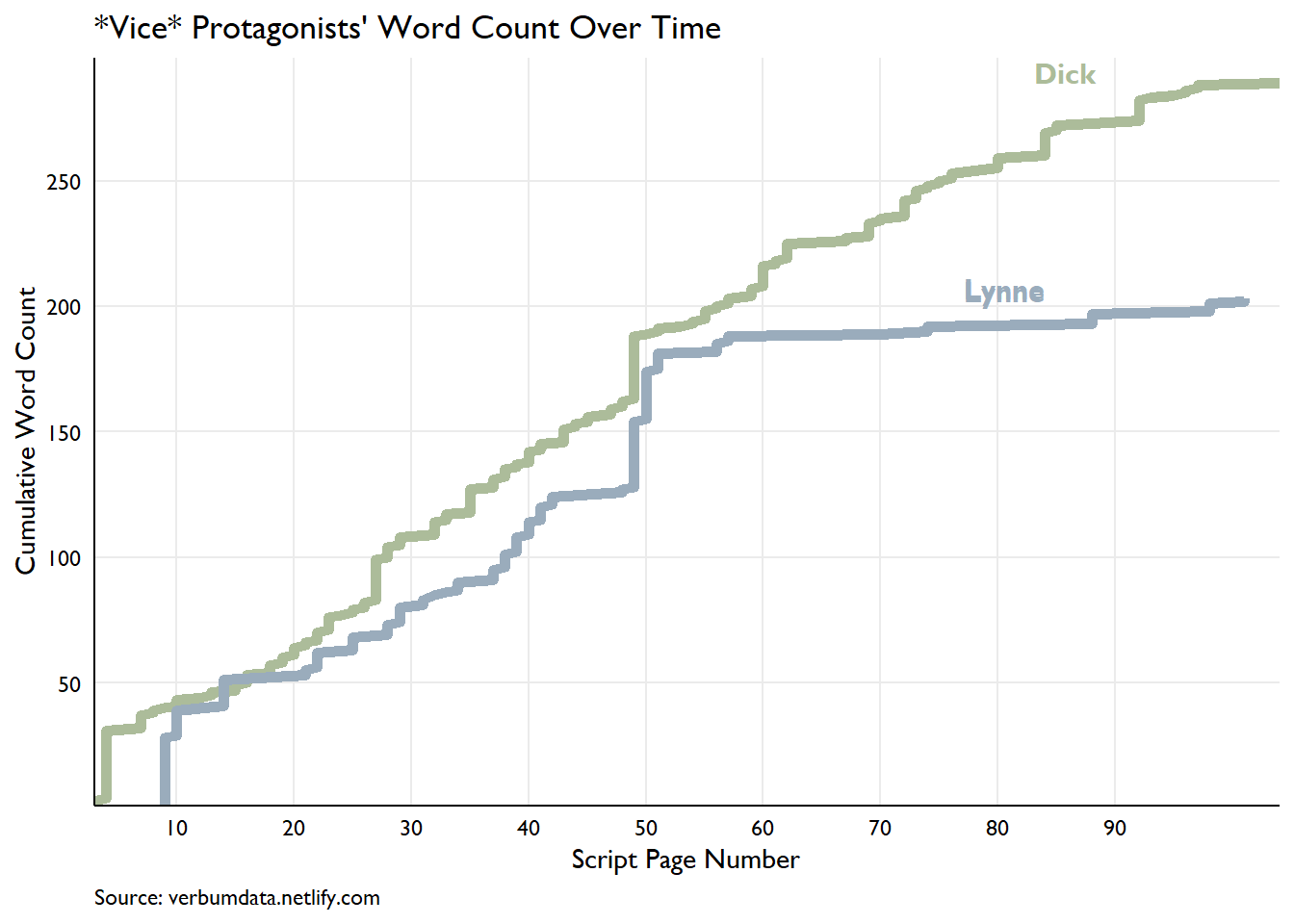

The movie becomes Dick’s movie. And Christian Bale makes us thankful for that. Hope you enjoyed this run through Vice. I would naturally encourage any and all to view.