This quick post was inspired by an Aaron Schatz tweet today which remarked on the quantitatively “best” team in the recent past:
He links to pro-football-reference.com. I took a gander and saw immediately that the website makes yards per play easily available.
As luck would have it, your author was lately preoccupied with just this statistic. 2018 NFL data I analyzed in the recent past show that a positive yards per play differential (at the game level) translates into a win about 70% of the time.
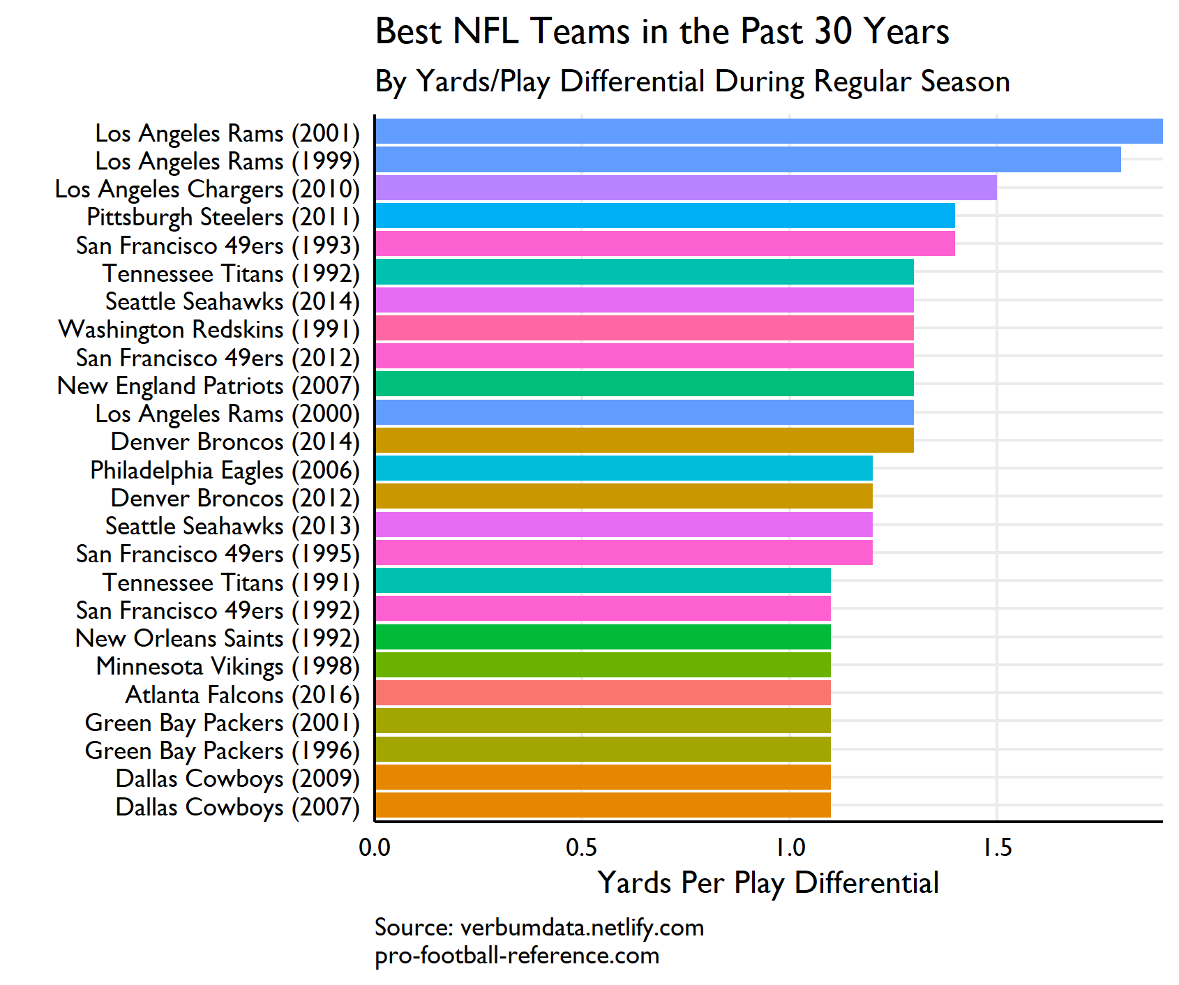
So why not look at the best teams of the last 30 years according to yards per play differential?!?
Here are the results (before the code):
How we got here…
First up are formalities of loading libraries and saving plot settings.
library(rvest)
library(tidyverse)
library(janitor)
library(extrafont)

# set theme

theme_set(
  theme_minimal(base_family = "Gill Sans MT") +
    theme(
      axis.line = element_line(color = "black"),
      axis.text = element_text(color = "black"),
      panel.grid.minor = element_blank(),
      plot.caption = element_text(hjust = 0)
    )
)
Now can proceed to the good stuff: web-scraping. To start the process, we will:
- Use
rvest::read_htmlto read in the relevant base website - Create our own links with each team’s abbreviation and the years from 1990-2019
- Celebrate
# get team abbreviations

team_abbs <- read_html("https://www.pro-football-reference.com/teams/")

links <- paste0(
  "https://www.pro-football-reference.com",
  team_abbs %>%
    html_nodes("a") %>%
    html_attr("href") %>%
    .[grepl("teams\\/[a-z]{3}\\/$", .)] %>%
    rep(2019-1990+1),
  sort(rep(1990:2019, 32)),
  ".htm"
)
Grab the data
We have the links. Now we need to write a function to take those links, scrape the data, and clean it up for us to evaluate.
# get best ypp differential w custom function

yppDiff <- possibly(

  function(link) {

  # read in html
  pg <- read_html(link)

  # extract stats of interest
  stats <- pg %>%
    html_nodes("table") %>%
    html_table() %>%
    .[[1]]

  # fix names and clean up df
  names(stats) <- unlist(ifelse(names(stats) == "", stats[1, ], paste(names(stats), stats[1, ], sep = "_")))
  stats <- clean_names(stats)
  names(stats)[names(stats) %in% c("tot_yds_to_ply", "tot_yds_to_y_p")] <- c("plays", "ypp")
  stats <- stats[-1, ]

  # add in team name & year

  stats$team <- str_extract(link, "(?<=teams\\/).+?(?=\\/)")
  stats$year <- str_extract(link, "\\d{4}")
  stats <- stats %>% select(team, year, everything())

  return(stats)

  },
  otherwise = NA_character_
)
With the function written, we can pipe it into execution. Now, before anyone complains about my for loop, I will tell you that from the violence of historical web-scraping, the loop is advantageous over base::lapply or purrr::map in only one respect: if it fails, you easily keep your progress. Yes, purrr trickery can save you, but this is so much easier…I also like the facility with which I can add a “counter” to check progress (I deleted it so it wouldn’t show on the post).
# get data

hist_data <- list()

for(i in seq_along(links)){
  hist_data[[i]] <- yppDiff(links[i])
}

# drop na & bind rows

hist_clean <- hist_data[!is.na(hist_data)] %>%
  bind_rows() %>%
  as_tibble()
Now, you’ll no doubt already know, but your author is lazy. Thus, I needed a quick mapping from the teams’ url abbreviations to human names. Thus the following chunk.
# now get team mapping

team_links <- links[grepl("2019", links)]

team_name <- possibly(
  function(link) {
    team_pg <- read_html(link)
    name <- team_pg %>%
      html_nodes("h1") %>%
      html_text() %>%
      str_remove_all("\n|\\s{3,}|\\d{4,}|Statistics & Players")

    df_out <- tibble(
      abbr = str_extract(link, "(?<=teams\\/).+?(?=\\/)"),
      name = name
    )

  },
  otherwise = NA_character_
)

team_lookup <- map_dfr(team_links, team_name)
YPP FTW
Now all the pieces can come together. We can positively determine the best teams of the past 30 years!
# find best ypp diff

ypp_rank <- hist_clean %>%
  filter(player %in% c("Team Stats", "Opp. Stats"),
         year != "2019") %>%
  select(team, year, player, ypp) %>%
  pivot_wider(
    names_from = "player",
    values_from = "ypp",
    names_repair = "universal"
  ) %>%
  mutate_at(vars(-team), list(as.numeric)) %>%
  mutate(ypp_diff = Team.Stats - Opp..Stats) %>%
  arrange(-ypp_diff) %>%
  slice(1:25) %>%
  left_join(team_lookup, by = c(team = "abbr")) %>%
  mutate(ypp_unique = paste0(name, " (", year, ")"))
And let’s plot.
ggplot(ypp_rank, aes(fct_reorder(ypp_unique, ypp_diff), ypp_diff)) +
  geom_col(show.legend = FALSE, aes(fill = team)) +
  coord_flip() +
  scale_y_continuous(expand = c(0,0)) +
  labs(x = "",
       y = "Yards Per Play Differential",
       title = "Best Teams in the Past 30 Years By Yards/Play Differential",
       caption = "Source: verbumdata.netlify.com\npro-football-reference.com")
The 2001 Rams of Kurt " don’t forget Jesus " fame top our list. What a fabulous team. Aaron’s 1996 Green Bay Packers arrive at 22nd on the list. Not too shabby, but not the best. Oh, and, PS, I dropped all 2019 data for sake of small sample.