Long time, no see. This will be a short one. The important thing here is to share a very useful trick for identifying matching elements across various strings. As shown below, this is particularly useful when you need to identify common variables across objects which are loosely, but not entirely, standardized.
What would a verbumdata post be without a teaser, though? Given the trick was discovered in the course of looking at building emissions data, I’ll share the best output of the day…More on that to close.
The reason for the post!
Often you might wish to identify common elements among various strings. R has no shortage of tools to conquer. But what if you are dealing with lists?
The workflow below shows a version of this problem where I was pulling Philly building emissions data across years and the columns for each year were not consistent. I wanted to find which columns were common to each dataframe and select only those.
First, we build a dataframe with our desired years and links.
library(tidyverse)
library(janitor)
library(extrafont)

links_philly <- tibble(
  year = as.character(2013:2018),
  link = c("https://data.phila.gov/carto/api/v2/sql?q=SELECT+*,+ST_Y(the_geom)+AS+lat,+ST_X(the_geom)+AS+lng+FROM+energy_usage_large_commercial_buildings_reported_2013&filename=energy_usage_large_commercial_buildings_reported_2013&format=csv&skipfields=cartodb_id",
           "https://phl.carto.com/api/v2/sql?q=select+*+from+energy_usage_large_commercial_buildings_reported_2014&format=csv&filename=energy_usage_large_commercial_buildings_reported_2014&skipfields=cartodb_id,the_geom,the_geom_webmercator",
           "https://phl.carto.com/api/v2/sql?q=SELECT+*+FROM+properties_reported_2015&filename=properties_reported_2015&format=csv&skipfields=cartodb_id,the_geom,the_geom_webmercator",
           "https://phl.carto.com/api/v2/sql?q=SELECT+*+FROM+properties_reported_2016&filename=properties_reported_2016&format=csv&skipfields=cartodb_id,the_geom,the_geom_webmercator",
           "https://phl.carto.com/api/v2/sql?q=SELECT+*+FROM+properties_reported_2017&filename=properties_reported_2017&format=csv&skipfields=cartodb_id,the_geom,the_geom_webmercator",
           "http://data-phl.opendata.arcgis.com/datasets/194499df063e43c7b95250e7eca41568_0.csv")
  )
Dirty, dirty links. Now, we map over our links, do a bit of cleaning (gracias janitor) and save it down.
# hoover it up!

philly_data <- map(links_philly$link, ~{read_csv(.x) %>% select_all(tolower)})
In an ideal world, each year would have the same fields. This is not an ideal world. Instead, here is what we face.
lapply(philly_data, names)## [[1]]
## [1] "the_geom"
## [2] "the_geom_webmercator"
## [3] "year_built"
## [4] "electricity_use_grid_purchase_and_generated_from_onsite_renewab"
## [5] "energy_star_score"
## [6] "portfolio_manager_id"
## [7] "water_use_all_water_sources_kgal"
## [8] "district_steam_use_kbtu"
## [9] "site_eui_kbtu_ft2"
## [10] "philadelphia_building_id"
## [11] "property_name"
## [12] "source_eui_kbtu_ft2"
## [13] "geom_address"
## [14] "fuel_oil_2_use_kbtu"
## [15] "number_of_buildings"
## [16] "property_floor_area_buildings_and_parking_ft"
## [17] "postal_code"
## [18] "natural_gas_use_kbtu"
## [19] "notes"
## [20] "total_ghg_emissions_mtco2e"
## [21] "primary_property_type_epa_calculated"
## [22] "lat"
## [23] "lng"
##
## [[2]]
## [1] "portfolio_manager_id"
## [2] "number_of_buildings"
## [3] "postal_code"
## [4] "property_name"
## [5] "source_eui_kbtu_ft"
## [6] "total_ghg_emissions_mtco2e"
## [7] "district_steam_use_kbtu"
## [8] "site_eui_kbtu_ft"
## [9] "primary_property_type_epa_calculated"
## [10] "natural_gas_use_kbtu"
## [11] "energy_star_score"
## [12] "location_1_address"
## [13] "year_built"
## [14] "fuel_oil_2_use_kbtu"
## [15] "property_floor_area_buildings_and_parking_ft"
## [16] "water_use_all_water_sources_kgal"
## [17] "electricity_use_kbtu"
## [18] "notes"
## [19] "philadelphia_building_id"
##
## [[3]]
## [1] "objectid" "portfolio_manager_id"
## [3] "street_address" "property_name"
## [5] "opa_account_num" "postal_code"
## [7] "num_of_buildings" "year_built"
## [9] "primary_prop_type_epa_calc" "total_floor_area_bld_pk_ft2"
## [11] "electricity_use_kbtu" "natural_gas_use_kbtu"
## [13] "fuel_oil_o2_use_kbtu" "steam_use_kbtu"
## [15] "energy_star_score" "site_eui_kbtuft2"
## [17] "source_eui_kbtuft2" "water_use_all_kgal"
## [19] "total_ghg_emissions_mtco2e" "notes"
##
## [[4]]
## [1] "objectid" "portfolio_manager_id"
## [3] "street_address" "property_name"
## [5] "opa_account_num" "postal_code"
## [7] "num_of_buildings" "year_built"
## [9] "primary_prop_type_epa_calc" "total_floor_area_bld_pk_ft2"
## [11] "electricity_use_kbtu" "natural_gas_use_kbtu"
## [13] "fuel_oil_o2_use_kbtu" "steam_use_kbtu"
## [15] "energy_star_score" "site_eui_kbtuft2"
## [17] "source_eui_kbtuft2" "water_use_all_kgal"
## [19] "total_ghg_emissions_mtco2e" "notes"
##
## [[5]]
## [1] "objectid" "portfolio_manager_id"
## [3] "street_address" "property_name"
## [5] "opa_account_num" "postal_code"
## [7] "num_of_buildings" "year_built"
## [9] "primary_prop_type_epa_calc" "total_floor_area_bld_pk_ft2"
## [11] "electricity_use_kbtu" "natural_gas_use_kbtu"
## [13] "fuel_oil_o2_use_kbtu" "steam_use_kbtu"
## [15] "energy_star_score" "site_eui_kbtuft2"
## [17] "source_eui_kbtuft2" "water_use_all_kgal"
## [19] "total_ghg_emissions_mtco2e" "notes"
##
## [[6]]
## [1] "objectid" "portfolio_manager_id"
## [3] "street_address" "property_name"
## [5] "opa_account_num" "zip_code"
## [7] "num_of_buildings" "year_built"
## [9] "primary_prop_type_epa_calc" "opa_square_footage"
## [11] "electricity_use_kbtu" "natural_gas_use_kbtu"
## [13] "fuel_oil_02_use_kbtu" "steam_use_kbtu"
## [15] "energy_star_score" "site_eui_kbtuft2"
## [17] "source_eui_kbtuft2" "water_use_all_kgal"
## [19] "total_ghg_emissions_mtco2e" "notes"
## [21] "x_coord" "y_coord"Not much in common there. Or, if there is anything in common, it is would take time (something which, dear reader, your lazy author spares not lightly) to idenitfy common elements.
Alas! Reduce to the rescue. This is the whole point of this post!
A very simple line of code helps you identify common column names across the list elements
Reduce(intersect, lapply(philly_data, names))## [1] "year_built" "energy_star_score"
## [3] "portfolio_manager_id" "property_name"
## [5] "natural_gas_use_kbtu" "notes"
## [7] "total_ghg_emissions_mtco2e"There you have it folks, the common set of elements you love to see!
More details on the leading plot…
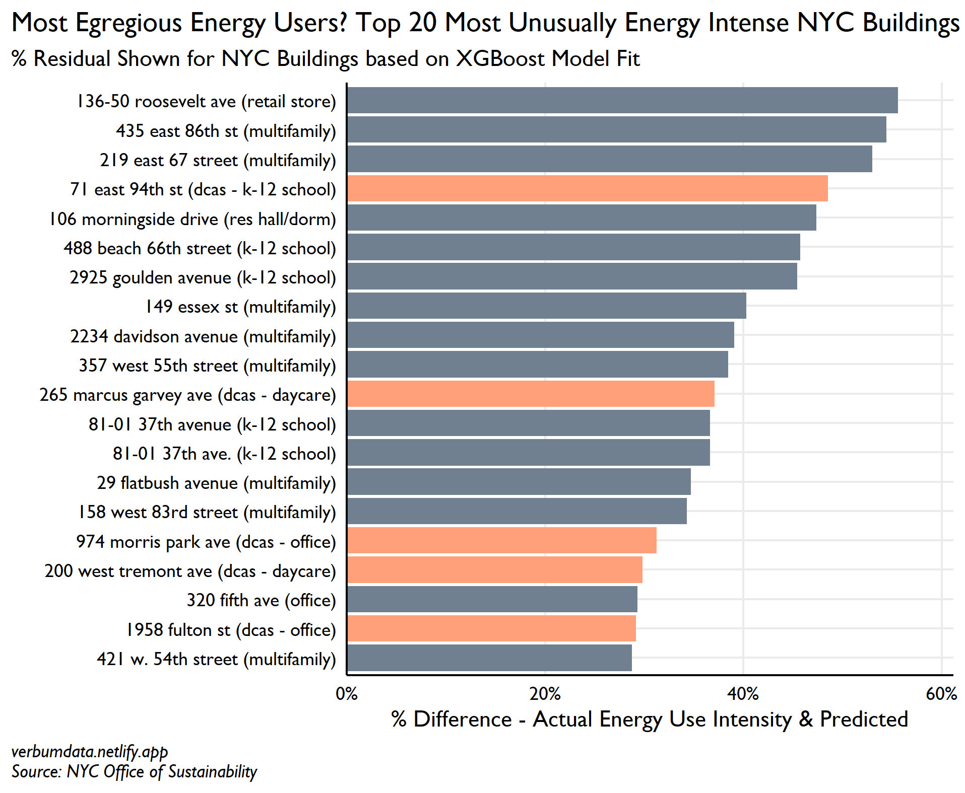
After taking down Philly, your author moved onto NYC. Long story short, I was interested in understanding which building out/underperform expectations in terms of energy use. I fit and XGBoost model to predict energy use and the plot at the top shows the largest outliers–i.e. those buildings whose actual energy use is farthest above their expected energy use.
First, a note. The salmon colored items are DCAS (NYC - Department of Citywide Administrative Services), the grey are private.
Weighing in at #1! The wonderful New World Mall in Flushing, NYC…worst underperformer in terms of energy use.