Computing COVID Bond Betas

Introducing the data

What have we here? We have a set of bond ETFs (with the obligatory S&P 500 comp) meant to crudely capture the array of fixed income markets. Introduction comes by the way of YTD 2020 returns (through 2020-11-20, as is everything here).

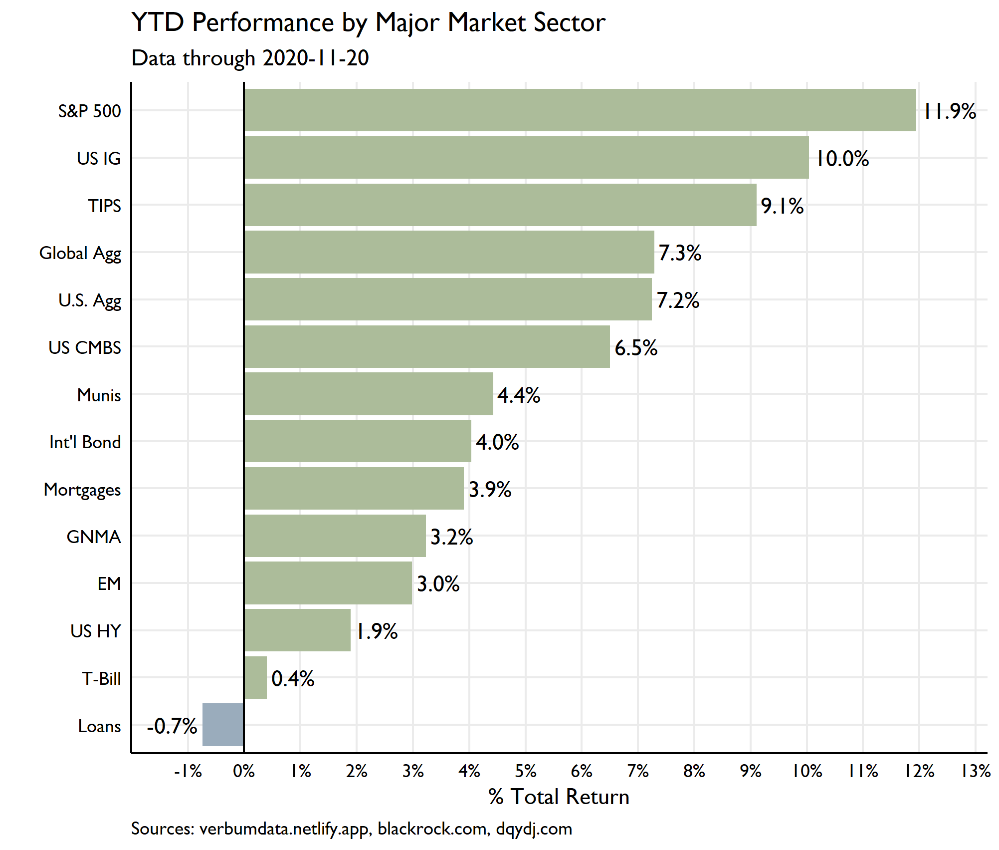
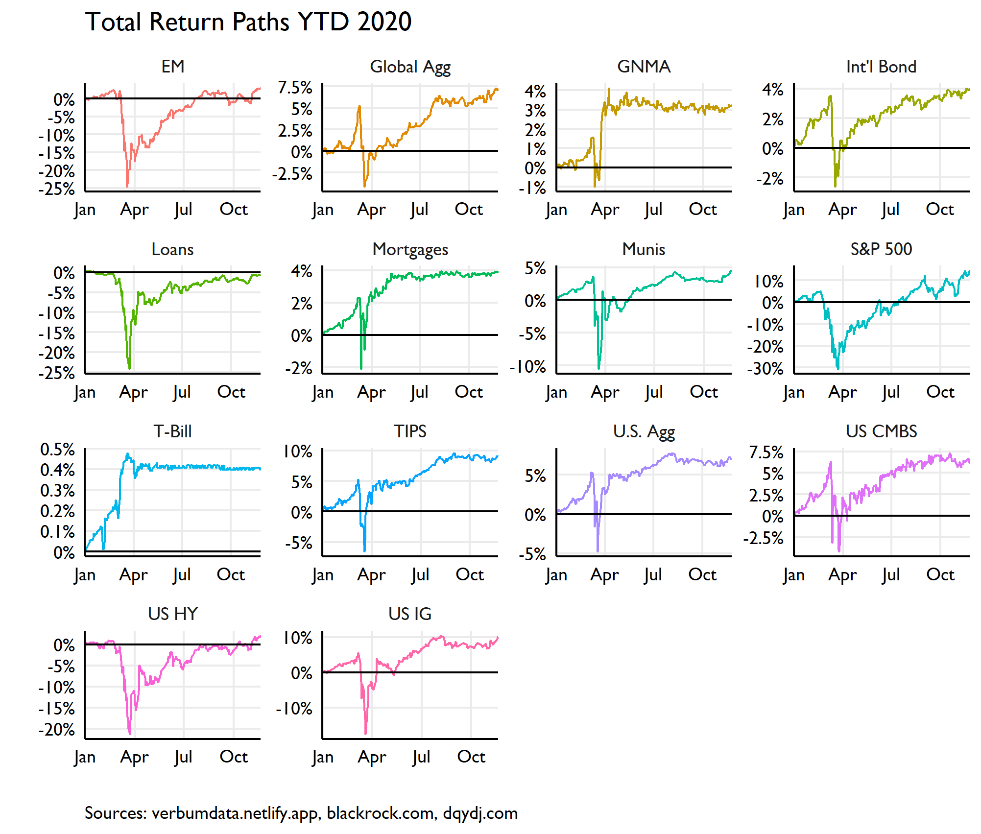
Bond ETFs will dominate this study. For sake of curiosity I included bank loans and the S&P. A short and incomplete explanatory summary of this sample would read: in 2020, returns revolved around friends of the Fed in duration nation. The paths of these returns are neat, too. Look at ol’ Ginnie Mae!!

Beta Mail

With the perfunctory introduction done, we now dive into the beta “replication” exercise. Unlike our dear friend RD (Reasonable Deviations d/b/a Robert Martin :)), I start here with outright beta calculations vs two indices. Part of the rationale behind computing two betas is to underscore how imperfect this exercise is. In the case of the betas calculated for the U.S. aggregate, we know !certainly! that some components are not even in the index (e.g. high yield and loans). This will complicate our later effort to isolate COVID effects.

The equation fit here is \[ R_{i,t}-R_{t}^f = a_i + \beta_i(R_{t}^m-R_{t}^f)+\epsilon_{i,t} \] where daily T-Bill returns are proxied by BIL. Yes they are insignificant-ish, and yes, I insisted on being neat, clean, and tidy.

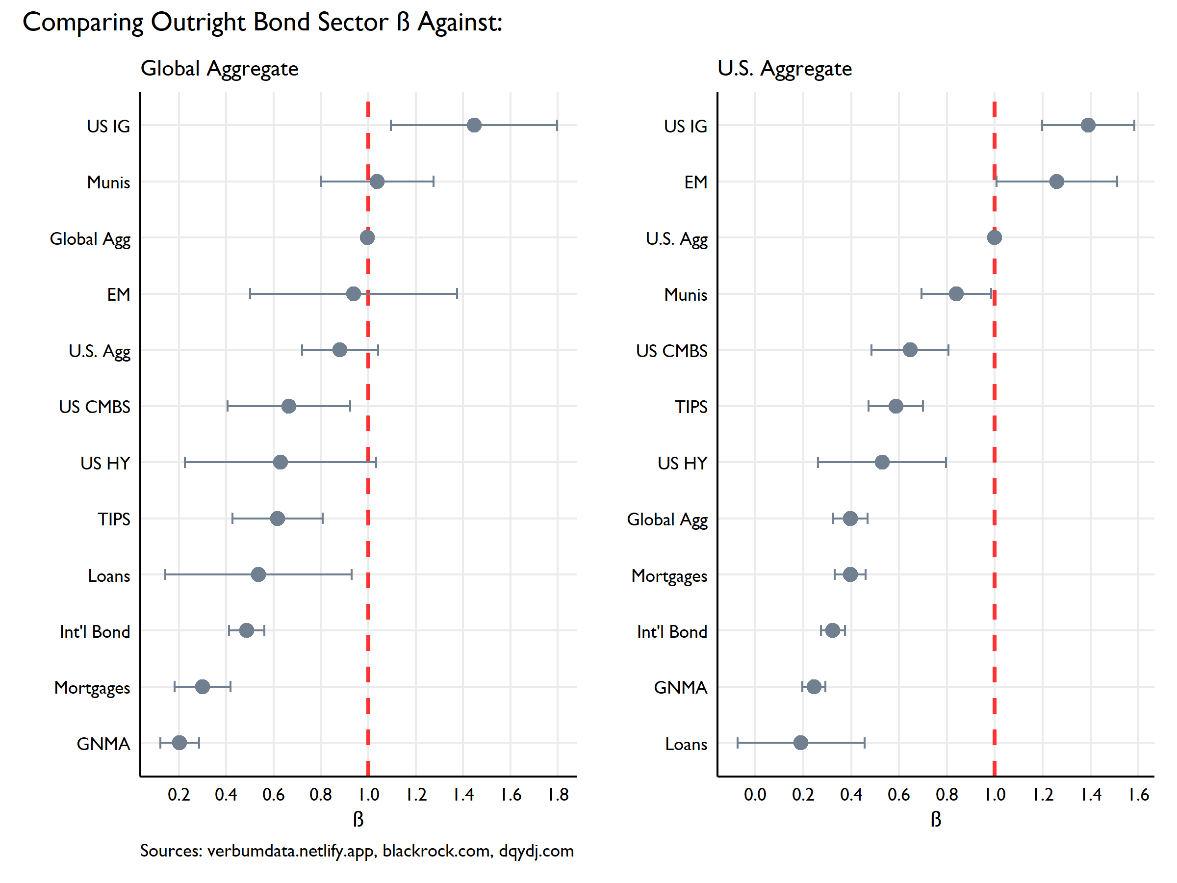
This plot shows the estimated beta for each sector against the respective index with confidence intervals (5th/95th) around the estimate. In the case of our global betas, many are not significantly different from 1.

Nevertheless, I see interesting threads on this here yarn. The sanity test is clean as US IG, on Gandalf’s the Fed’s winged Eagles, flies high. Also sporting a beta > 1 (just barely) is EM. Counterintuitive though it may be, the $ is the world’s reserve currency and so easy $ financing via the Fed bleeds into the already volatile EM sector.

I’d venture to guess the low beta of international bonds vis-à-vis the global Agg is explained largely by the absence of U.S. assets in the ETF and the dominance of U.S. assets in the global agg (~1/3 of the assets are U.S.).

Also, for the curious, the U.S. Agg beta vs the Global Agg and the Global Agg beta vs the U.S. Agg are not equal because the intercept (alpha) is non-zero, though statistically insignificant.

COVID Betas

Now into the good stuff. For sake of ease–and likely honesty–we will restrict ourselves here to controlling for the U.S. Agg only as the beta estimates are unsurprisingly cleaner (just have a look at those confidence intervals).

My methodology here is slightly different to dear Robert’s. In the first instance, I’ve used the daily percent change in U.S. COVID-reported deaths rather than case counts. Thinking goes that death counts are less but not un- biased overtime by changes in reporting methodologies and testing velocity. One hopes these estimates are ever so slightly more stable into the future.

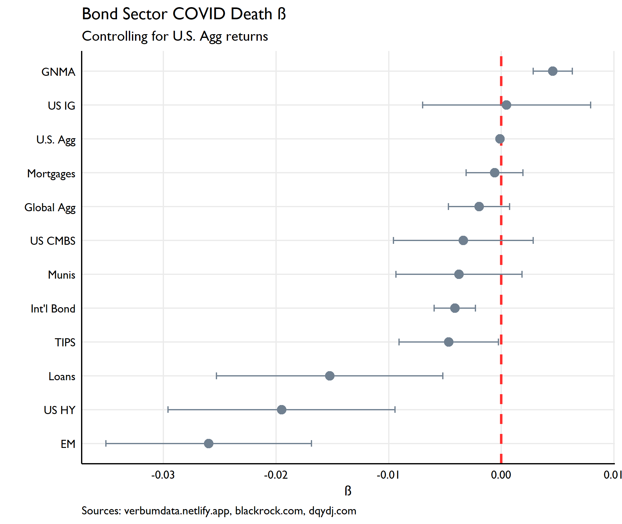
Wow momma! This is neat. What we see are the effects of policy changes on the plus-ish side, (GNMA forbearance, Fed intervention) and heavy risk off sectors scarred by higher death counts. In truth, I’d say the negative lessons here have more to do with the effect outliers have on biasing data (looking at you risk-on sectors).

The great swath of unwashed betas not distinguishable from zero show the mixed bag. CMBS and Munis lean negative as COVID has throw ~1/12th of the commercial mortgage market into serious delinquency and has put many municipal budgets through a grater. Mortgages more generally have benefited from some policy mitigants, but have had also to contend with heavy prepay dynamics and broader distopian ricochet on display in the U.S. housing market.

Wrap it up!

I don’t expect these results to be robust enough to trade on or around. Similar to anything on this here blog, none of these studies should be construed as investment advice and only represent your author’s own uncannily fallacious thinking. That said, I do think that the rebound in EM, HY, and Loans (along w/ TIPS??) is a result which would shock few.

Perhaps the more interesting dynamic will be the evolution of spreads (and total returns) in U.S. IG. Continued recovery and broader risk on argue for tighter spreads. The removal of the Fed’s explicit support for the market argues for wider spreads (true too for secondary CMBS and other sectors which benefited from the many and varied policy actions). Mean reversion should be expected, I think, in line with normalization of the betas observed in the outright study above.

Thanks for reading! Code below:

# import libraries

library(jsonlite)
library(tidyverse)
library(lubridate)
library(janitor)
library(extrafont)
library(readxl)
library(patchwork)

# set theme

theme_set(
  theme_minimal(base_family = "Gill Sans MT") +
    theme(axis.line = element_line(color = "black"),
          axis.text = element_text(color = "black"),
          axis.title = element_text(color = "black"),
          panel.grid.minor = element_blank(),
          plot.caption = element_text(hjust = 0)
          )
)

ticks_bond <- tibble(
  fund_name = c(sprintf("iShares %s Bond ETF", 
                      c("GNMA", "CMBS", "iBoxx $ Investment Grade Corporate",
                        "iBoxx $ High Yield Corporate", "MBS", "TIPS", 
                        "National Muni", "J.P. Morgan USD Emerging Markets", 
                        "Core U.S. Aggregate", "Core Int'l Aggregate")), "Invesco Senior Loan ETF","S&P 500", "SPDR Barclays 1-3mo T-Bill ETF"),
  ticker = c("GNMA", "CMBS", "LQD", "HYG", "MBB", "TIP", "MUB", "EMB","AGG", "IAGG", "BKLN", "SPY", "BIL"),
  asset_class = c("GNMA", "US CMBS", "US IG", "US HY", "Mortgages", "TIPS", "Munis", "EM", "U.S. Agg", "Int'l Bond", "Loans", "S&P 500", "T-Bill")
)

# get nyt covid data

nyt_covid <- read_csv("https://raw.githubusercontent.com/nytimes/covid-19-data/master/us.csv") %>% 
  mutate(date = as.Date(date))

# function to get etf data and calc total return

etf_ts_data <- function(ticker) {
  
  message(sprintf("Getting YTD total return data for %s ...", ticker))
  
  # api limit is 10 per second, 50 per day
  Sys.sleep(10)
  
  link <- sprintf("https://timeseries.apps.dqydj.com/timeseries/item/%s?begin_date=2019-12-31&end_date=2020-11-26&type=exchange_traded_fund", ticker)
  json_data <- fromJSON(link)
  clean_json <- fromJSON(json_data$history) %>% 
    as_tibble() %>% 
    select(date, close, dividend) %>% 
    mutate(date = as.Date(as_datetime(date / 1000)),
           ticker = ticker,
           dividend_pay = lag(dividend, 4),
           dividend_pay = ifelse(is.na(dividend_pay), 0, dividend_pay),
           div_share = dividend_pay / close,
           share_owned = 1 + cumsum(div_share),
           pos_value = share_owned * close,
           daily_ret = pos_value / lag(pos_value, 1) - 1,
           daily_ret = ifelse(is.na(daily_ret), 0, daily_ret),
           tot_ret_idx = cumprod(1 + daily_ret))
}

# now get ze mkt data

mkt_data <- map_dfr(ticks_bond$ticker, etf_ts_data)

# but we need the blackrock agg data b/c it is a ucit & isn't on the IEX api,
# you can find it here https://www.blackrock.com/americas-offshore/products/291773/fund

blackrock_aggg_data <- readRDS("/2020-11-27_aggg-performance-data.rds")

perf <- blackrock_aggg_data %>% 
  mutate(as_of = mdy(as_of),
         fund_return_series = as.numeric(fund_return_series)) %>% 
  filter(as_of >= "2019-12-31") %>% 
  arrange(as_of) %>% 
  mutate(daily_ret = fund_return_series / lag(fund_return_series, 1) - 1,
         daily_ret = ifelse(is.na(daily_ret), 0, daily_ret),
         tot_ret_idx = cumprod(1 + daily_ret),
         ticker = "AGGG",
         asset_class = "Global Agg") %>% 
  select(date = as_of, ticker, daily_ret, tot_ret_idx)

# put it all together

mkt_data_full <- mkt_data %>% 
  bind_rows(perf) %>% 
  left_join(ticks_bond, by = c("ticker")) %>% 
  mutate(asset_class = ifelse(ticker == "AGGG", "Global Agg", asset_class))

### plotting and data

# overall returns

returns <- mkt_data %>% 
  select(date, ticker, tot_ret_idx) %>% 
  bind_rows(perf %>% select(-daily_ret)) %>% 
  left_join(ticks_bond, by = c("ticker")) %>% 
  mutate(asset_class = ifelse(ticker == "AGGG", "Global Agg", asset_class))
  
# top performers

ytd <- returns %>% 
  group_by(ticker) %>% 
  arrange(desc(date)) %>% 
  filter(date == "2020-11-20") %>% 
  mutate(tot_ret_idx = (tot_ret_idx - 1) * 100)

  
ggplot(ytd, aes(fct_reorder(asset_class, tot_ret_idx), tot_ret_idx)) +
  geom_col(aes(fill = tot_ret_idx > 0), show.legend = FALSE) +
  geom_hline(yintercept = 0) +
  geom_text(aes(label = sprintf("%1.1f%%", tot_ret_idx)),
            hjust = ifelse(ytd$tot_ret_idx < 0, 1.1, -0.1),
            show.legend = FALSE,
            family = "Gill Sans MT") +
  scale_fill_manual(values = c("#9aacbc", "#acbc9a")) +
  scale_y_continuous(breaks = seq(-1, 13, 1), 
                     labels = function(x) sprintf("%.0f%%", x),
                     expand = c(0.1,0,0.1,0)) +
  coord_flip() +
  labs(title = "YTD Performance by Major Market Sector",
       subtitle = "Data through 2020-11-20",
       x = "",
       y = "% Total Return",
       caption = "Sources: verbumdata.netlify.app, blackrock.com, dqydj.com")

# return paths

returns %>% 
  mutate(tot_ret_idx = (tot_ret_idx - 1) * 100) %>% 
  ggplot(aes(date, tot_ret_idx, color = asset_class)) +
  geom_line(show.legend = FALSE) +
  geom_hline(yintercept = 0) +
  scale_y_continuous(labels = function(x) paste0(x, "%")) +
  scale_x_date(expand = c(0,0,0,0)) +
  facet_wrap(~ asset_class, scales = "free") +
  labs(x = "",
       y = "",
       title = "Total Return Paths YTD 2020",
       caption = "Sources: verbumdata.netlify.app, blackrock.com, dqydj.com")

# data to bind for regression

agg_spy <- mkt_data_full %>% 
  filter(ticker %in% c("SPY", "AGG", "AGGG", "BIL")) %>% 
  mutate(ticker = tolower(ticker)) %>% 
  pivot_wider(date, names_from = "ticker", names_prefix = "daily_ret_", values_from = "daily_ret")


# create regression data

regression_data <- mkt_data_full %>% 
  filter(date < "2020-11-21") %>% 
  left_join(nyt_covid, by = "date") %>% 
  left_join(agg_spy, by = "date") %>% 
  mutate(across(c(cases, deaths), ~ replace_na(.x / lag(.x, 1) - 1, 0), .names = "{col}_chg"),
         across(where(is.numeric), ~ ifelse(is.infinite(.x), 0, .x)))

# outright beta

outright_beta_agg <- regression_data %>% 
  group_by(asset_class) %>% 
  group_modify(~ broom::tidy(lm((daily_ret - daily_ret_bil) ~ (daily_ret_agg - daily_ret_bil), data = .x), conf.int = TRUE)) %>% 
  filter(term != "(Intercept)" & !asset_class %in% c("S&P 500", "T-Bill"))

agg_b_plot <- ggplot(outright_beta_agg, aes(estimate, fct_reorder(asset_class, estimate))) +
  geom_vline(xintercept = 1, color = "firebrick1", lty = 2, size = 1) +
  geom_point(size = 3, color = "slategrey") +
  geom_errorbar(aes(xmin = conf.low, xmax = conf.high), 
                width = 0.2,
                color ="slategrey") +
  scale_x_continuous(breaks = seq(0.0, 1.6, 0.2)) +
  labs(x = "β",
       y = "",
       subtitle = "U.S. Aggregate")


outright_beta_aggg <- regression_data %>% 
  group_by(asset_class) %>% 
  group_modify(~ broom::tidy(lm((daily_ret - daily_ret_bil) ~ (daily_ret_aggg - daily_ret_bil), data = .x), conf.int = TRUE)) %>% 
  filter(term != "(Intercept)" & !asset_class %in% c("S&P 500", "T-Bill"))

aggg_b_plot <- ggplot(outright_beta_aggg, aes(estimate, fct_reorder(asset_class, estimate))) +
  geom_vline(xintercept = 1, color = "firebrick1", lty = 2, size = 1) +
  geom_point(size = 3, color = "slategrey") +
  geom_errorbar(aes(xmin = conf.low, xmax = conf.high), 
                width = 0.2,
                color ="slategrey") +
  scale_x_continuous(breaks = seq(0.2, 1.8, 0.2)) +
  labs(x = "β",
       y = "",
       subtitle = "Global Aggregate",
       caption = "Sources: verbumdata.netlify.app, blackrock.com, dqydj.com")

aggg_b_plot + 
  agg_b_plot + 
  plot_annotation("Comparing Outright Bond Sector β Against:")

# beta w covid

covid_beta <- regression_data %>% 
  group_by(asset_class) %>% 
  group_modify(~ broom::tidy(lm((daily_ret - daily_ret_bil) ~ (daily_ret_agg - daily_ret_bil) + deaths_chg, data = .x), conf.int = TRUE)) %>% 
  filter(term == "deaths_chg" & !asset_class %in% c("S&P 500", "T-Bill"))

ggplot(covid_beta, aes(estimate, fct_reorder(asset_class, estimate))) +
  geom_vline(xintercept = 0, color = "firebrick1", lty = 2, size = 1) +
  geom_point(size = 3, color = "slategrey") +
  geom_errorbar(aes(xmin = conf.low, xmax = conf.high), 
                width = 0.2,
                color ="slategrey") +
  scale_x_continuous(breaks = seq(-0.05, 0.05, 0.01)) +
  labs(x = "β",
       y = "",
       title = "Bond Sector COVID Death β",
       subtitle = "Controlling for U.S. Agg returns")