Fumble Mumble Jumble

How many fumbles should we expect?

There are two approaches we might take to estimate the number of fumbles one should expect any given Sunday:

• Method 1: Model fumbles per game
• Method 2: Model fumbles per Sunday

Given the variability in the number of games played per Sunday (and the fact not all games have been played), we use method 1.

First, we get the data from the still wonderful nflscrapR-data repo. For those sleeping, the nflscrapR package broke as the NFL fettered API access. Nevertheless, we can use the repo to model fumbles per game from 2009-2019.

I’m counting all fumbles in a regular season or post-season game, regardless of whether they were lost.

# load libraries

library(tidyverse); library(data.table)
library(extrafont); library(lubridate)
library(rvest)

theme_set(
  theme_minimal(base_family = "Gill Sans MT") +
    theme(axis.line = element_line(color = "black"),
          axis.text = element_text(color = "black"),
          axis.title = element_text(color = "black"),
          panel.grid.minor = element_blank(),
          plot.caption = element_text(hjust = 0)
          )
)

# create links for regular season and post season play by play data

reg_links <- sprintf("https://raw.githubusercontent.com/ryurko/nflscrapR-data/master/play_by_play_data/regular_season/reg_pbp_%d.csv", 2009:2019)
pos_links <- sprintf("https://raw.githubusercontent.com/ryurko/nflscrapR-data/master/play_by_play_data/post_season/post_pbp_%d.csv", 2009:2019)

# pull the data and combine

reg_pbp <- map_dfr(reg_links, fread)
pos_pbp <- map_dfr(pos_links, fread)
nfl_hist <- bind_rows(reg_pbp, pos_pbp)

# get the counts

fumbles <- nfl_hist %>% 
  group_by(game_id) %>% 
  summarize(total_fumbles = sum(fumble, na.rm = T))

# fumbles per game

ggplot(fumbles, aes(total_fumbles)) +
  geom_histogram(color = "white", fill = "#9aacbc", binwidth = 1) +
  scale_y_continuous(expand = c(0,0,0.1,0)) +
  scale_x_continuous(breaks = seq(0, 11, 1)) +
  labs(x = "Fumbles",
       y = "Game Count",
       title = "NFL Fumbles Per Game",
       subtitle = paste0("Data from (Regular|Post) Seasons 2009-2019\n", 
                         "Mean = ", round(mean(fumbles$total_fumbles), 1), 
                         " | Median = ", median(fumbles$total_fumbles)))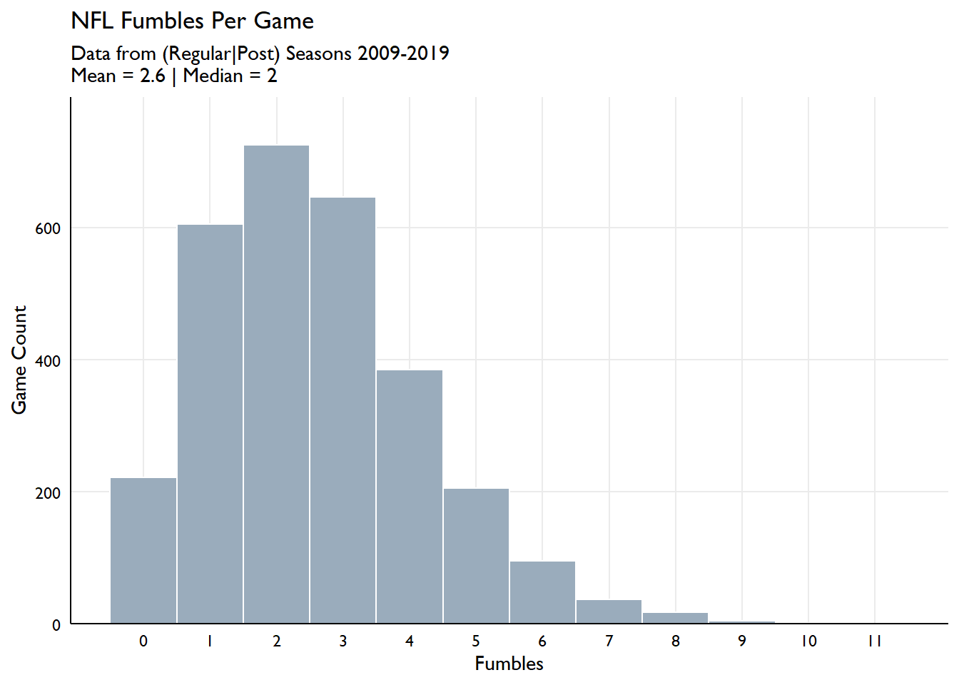

Cool distribution. Readers of the blog should be familiar with this distribution as we saw it in a prior post, looking at hockey goals per game.

For the insatiably curious, the game which featured the most fumbles was a game played on 2020-09-19 in Nashville, TN between the Steelers and the Titans. The Titans fumbled 7! times and the Steelers fumbled 4 times.

Model it up

Now that we know what we are looking for, we can model the # of fumbles per game as a Poisson process.

# compare distributions

fpg <- fumbles %>% 
  count(total_fumbles, name = "actual") %>% 
  arrange(total_fumbles) %>% 
  mutate(pois = dpois(total_fumbles, mean(fumbles$total_fumbles)) * sum(actual))

fpg %>% 
  setNames(c("total_fumbles", "Actual Fumbles", "Poisson Modeled Fumbles")) %>% 
  pivot_longer(-total_fumbles, names_to = "type", values_to = "value") %>% 
  ggplot(aes(total_fumbles, value, fill = type)) +
  geom_bar(stat = "identity", position = "dodge") +
  scale_fill_manual(values = c("#acbc9a", "#9aacbc")) +
  scale_y_continuous(expand = c(0,0,0.1,0)) +
  scale_x_continuous(breaks = seq(0, 11, 1)) +
  labs(x = "Fumbles",
       y = "Game Count",
       title = "NFL Fumbles Per Game",
       subtitle = paste0("Data from (Regular|Post) Seasons 2009-2019\n"),
       caption = "Sources: verbumdata.netlify.app, nflscrapR-data, footballdb.com") +
  theme(legend.position = "top",
        legend.title = element_blank(),
        legend.key.size = unit(0.75, "line"))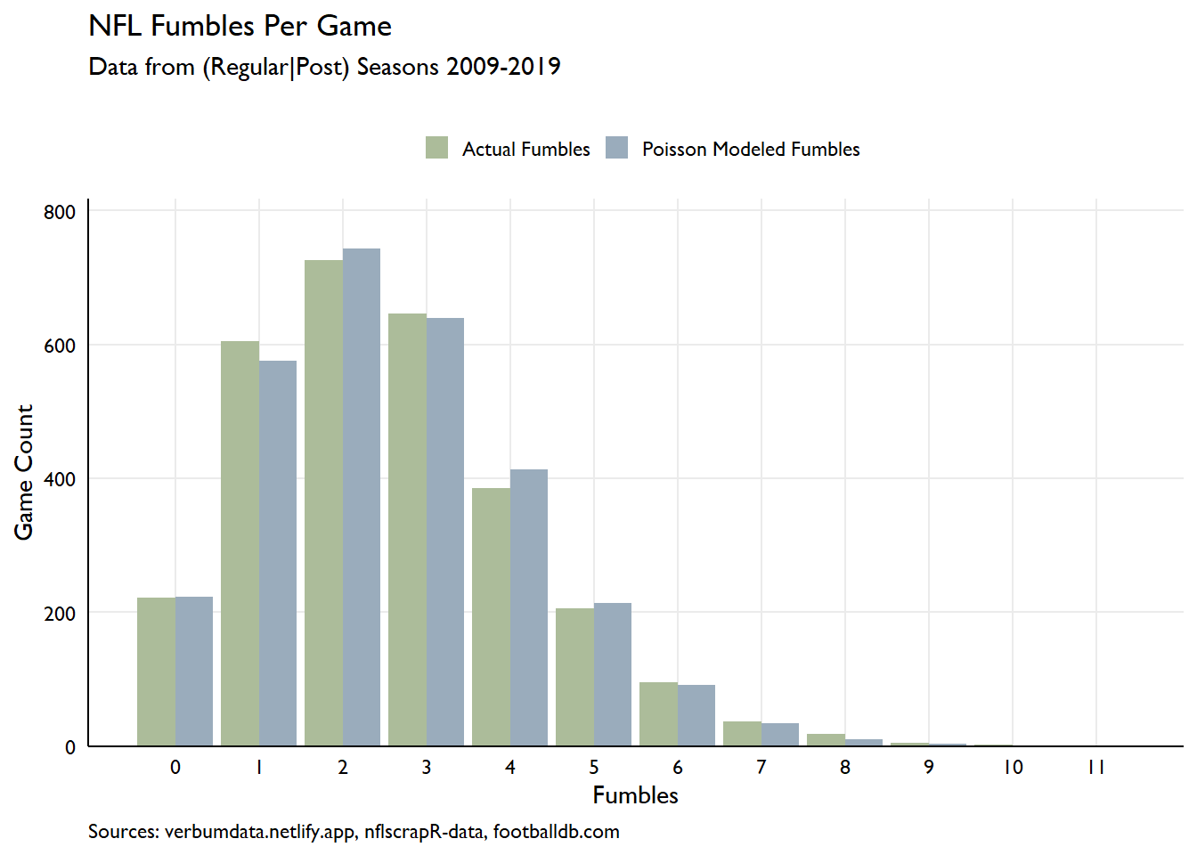

Let’s get today’s fumble count to compare. You might notice here the advent of the often maligned for loop in R. I’d advise those who would otherwise not wrap their function in purrr::possibly (see an old post here for details) to utilize loops when we scraping. If things go wrong, you don’t lose the whole lot!

# get fumbles today

pg <- read_html("https://www.footballdb.com/games/index.html")

today_game_links <- pg %>% 
  html_nodes("a") %>% 
  html_attr("href") %>% 
  .[grepl(format(Sys.Date(), "%Y%m%d"), .)] %>% 
  paste0("https://www.footballdb.com", .)

get_fumble_counts <- function(link) {
  
  pg <- read_html(link)
  
  game <- pg %>% 
  html_nodes("h1") %>% 
  html_text()
  
  message(sprintf("Getting fumble counts for %s", game))
  
  box <- pg %>% 
    html_nodes("table") %>% 
    html_table() %>% 
    .[grepl("Fumbles", .)]
  
  fumb <- box[[1]] %>% 
  .[grepl("Fumbles", .$X1), 2:3]
  
  tibble(
    game = game,
    fumbles = sum(as.numeric(sapply(strsplit(as.character(fumb), "-"), "[[", 1)))
  )
  
}
# allocate vector and run

fum_counts <- list()

for(i in seq_along(today_game_links)) {
  fum_counts[[i]] <- get_fumble_counts(today_game_links[i])
}

fumbles_today <- bind_rows(fum_counts)

Poisson fits the data very well! With this in hand, we can estimate the number of fumbles we’d expect to see based on the distribution. Some fast calculating shows that the 11 games played so far on Sunday November 29th, 2020 have produced 29 fumbles.

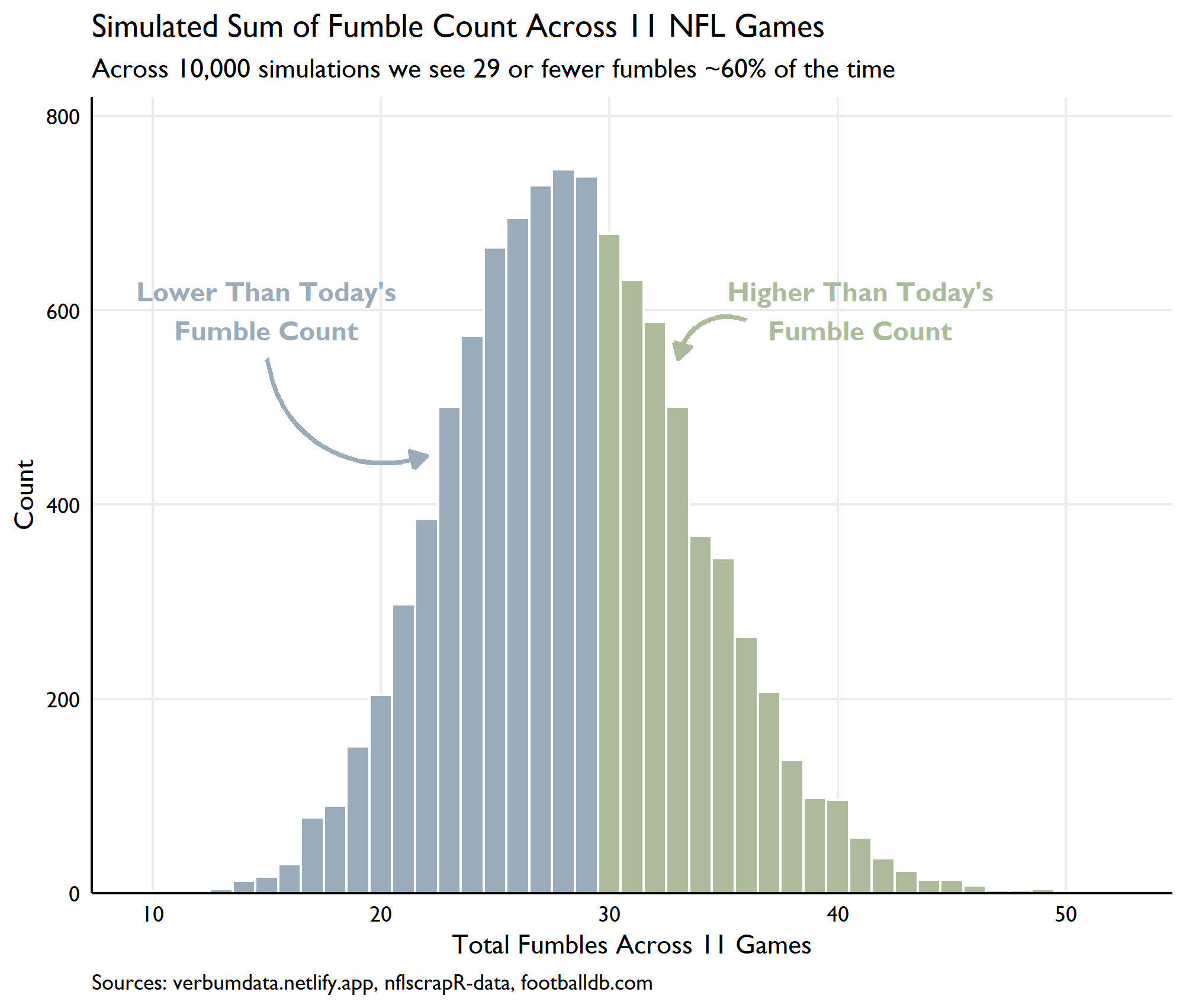
So, how likely is this result? Imagine we played today’s 11 games 10,000 times…how many fumbles should we expect?

# play the darn thing 100,000 times

play_sunday <- tibble(
  sim_no = 1:10000,
  fumbles = replicate(10000, sum(rpois(11, lambda = mean(fumbles$total_fumbles)))),
  is_less = fumbles <= sum(fumbles_today$fumbles)
)

Excluding the Packers/Bears game, across 11 NFL games, we’d expect 29 or more fumbles 41.10% of the time. Not so bad, but not a massive outlier. Check out the breakdown below.

# play the darn thing 100,000 times

ggplot(play_sunday, aes(fumbles, fill = is_less), color = "dummy") +
  geom_histogram(binwidth = 1, color = "white", show.legend = FALSE) +
  scale_fill_manual(values = c("#acbc9a", "#9aacbc")) +
  scale_color_manual(values = c("#acbc9a", "#9aacbc"), labels = c("FALSE", "TRUE")) +
  scale_y_continuous(expand = c(0,0,0.1,0)) +
  annotate("text", x = 15, y = 600, 
           label = "Lower Than Today's\nFumble Count",
           hjust = 0.5,
           family = "Gill Sans MT",
           color = "#9aacbc",
           fontface = "bold") +
  annotate("text", x = 41, y = 600, 
           label = "Higher Than Today's\nFumble Count",
           hjust = 0.5,
           family = "Gill Sans MT",
           color = "#acbc9a",
           fontface = "bold") +
  geom_curve(aes(x = 15, xend = 22, 
                 y = 550, yend = 450),
               color = "#9aacbc",
               size = 1,
               arrow = arrow(length = unit(0.25, "cm"), type = "closed")) +
  geom_curve(aes(x = 36, xend = 33, 
                 y = 590, yend = 550),
               color = "#acbc9a",
               size = 1,
               arrow = arrow(length = unit(0.25, "cm"), type = "closed")) +
  labs(x = "Total Fumbles Across 11 Games",
       y = "Count",
       fill = "",
       title = "Simulated Sum of Fumble Count Across 11 NFL Games",
       subtitle = "Across 10,000 simulations we see 29 or fewer fumbles 60% of the time",
       caption = "Sources: verbumdata.netlify.app, nflscrapR-data, footballdb.com") +
   theme(
     legend.position = "top",
     legend.key.size = unit(0.75, "line"),
     legend.justification = "center"
     )

For the statistically inclined, we can see the central limit theorem here in action. Repeated samples from our poisson process produce a very clean normal distribution!