It’s the most wonderful time of the year. The Census releases their 5-Year ACS estimates each time around this year, revealing trends afoot in our most wonderful United States of America. These estimates are broader (smaller areas covered) and are more stable estimates. Here’s the official release announcement.
First question to answer, and the subject of this blog post. Which metro areas have seen their populations burgeon as a result of out of state/out of country new movers?
Well, without further ado, here’s your answer!
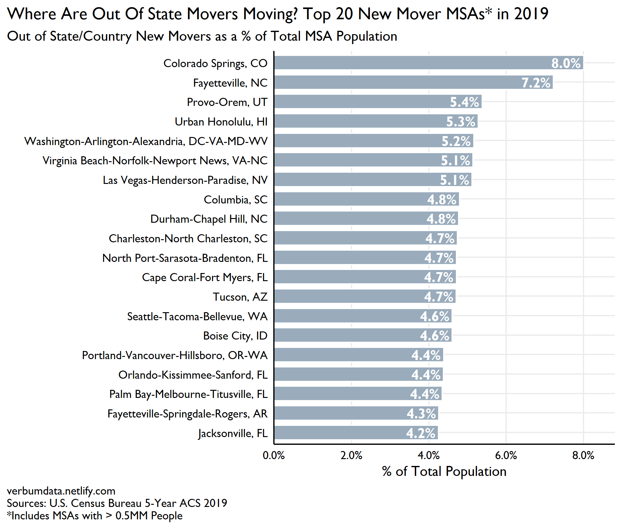
Shocking to think that nearly 1 in 12 Colorado Springians is fresh off the proverbial boat (well, I guess they could have driven…).
This begs a natural question, one which the delights of tidycensus make us well prepared to answer. What would a map show?
Alas! The answer:
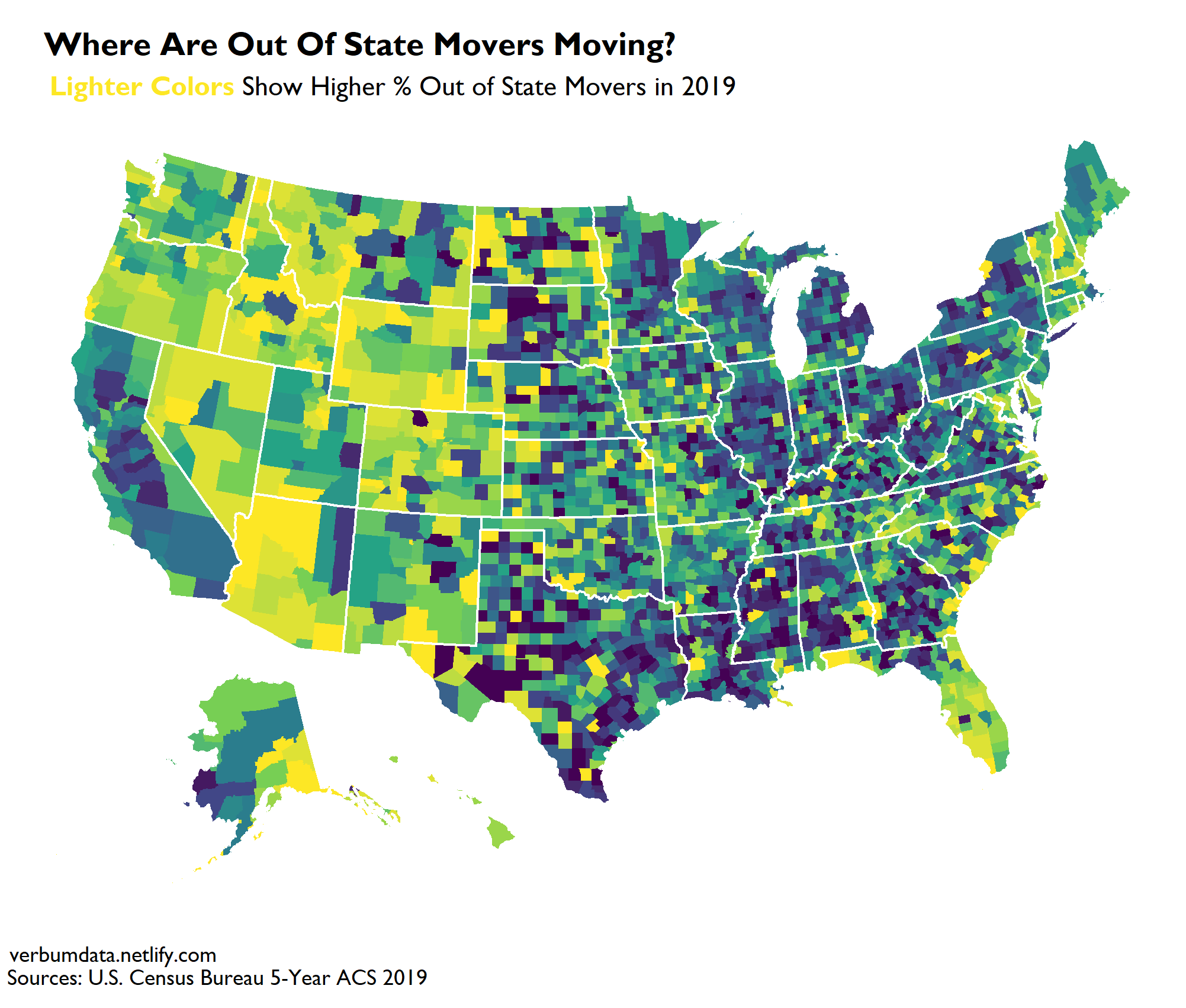
Major trends to observe? Hopefully the map makes trends abundantly clear!
- California, NYC, much of rural America and the Midwest are not attracting out of state movers
- Nevada, Arizona, Wyoming, Colorado, Florida and North Dakota saw lots of out of state movers in 2019
A few notes here needed on methodology. Unlike our MSA table, this map shows counties (make the mapping easier). To generate the colors, the county-level share of out of state movers were sorted into 20 buckets and colored accordingly.
Perhaps more to come on this data in the future? Thanks for reading!! Code below for the curious.
library(tidycensus)
library(tidyverse)
library(extrafont)
library(sf)
library(usmap)
library(ggtext)

# set theme

theme_set(
  theme_minimal(base_family = "Gill Sans MT") +
    theme(axis.line = element_line(color = "black"),
          axis.text = element_text(color = "black"),
          axis.title = element_text(color = "black"),
          panel.grid.minor = element_blank(),
          plot.caption = element_text(hjust = 0)
    )
)

# set census key & tigris options

census_api_key(Sys.getenv("CENSUS_API_KEY"))
options(tigris_use_cache = TRUE)

# get variables

lookup_vars <- load_variables(year = 2019, dataset = "acs1", cache = TRUE)

# filter my relevant data

pop_vars <- lookup_vars %>%
  filter(str_detect(name, "B07001")) %>%
  mutate(label = str_remove_all(label, "Estimate!!Total!!")) %>%
  select(variable = name, demographic = label)

# get population info

years_of_int <- 2012:2019

acs_import <- map_df(
  years_of_int,
  ~ get_acs(
    geography = "metropolitan statistical area/micropolitan statistical area",
    table = "B07001",
    year = .x,
    survey = "acs5",
    cache_table = TRUE
  ),
  .id = "year"
) %>%
  mutate(year = min(years_of_int) - 1 + as.numeric(year)) %>%
  filter(!is.na(estimate))

# datasets for geometry

geo_data <- get_acs(
  geography = "county",
  variable = c("B07001_001", "B07001_065", "B07001_081"),
  year = 2019,
  geometry = TRUE,
  shift_geo = TRUE
)

state_geo <- get_acs(
  geography = "state",
  variable = "B07001_001",
  year = 2019,
  geometry = TRUE,
  shift_geo = TRUE
)

# clean population info

clean_pop <- acs_import %>%
  select_all(tolower) %>%
  select(-geoid) %>%
  left_join(popVars, by = "variable") %>%
  mutate(
    variable = str_extract(demographic, "(?<=:!!).+?(?=:)"),
    variable = if_else(is.na(variable), "Total", variable),
    age = str_extract(demographic, "(?<=:!!)\\d+.*"),
    age = if_else(is.na(age), "Total", age),
    name = ifelse(name %in% "Texarkana, TX-Texarkana, AR Metro Area", "Texarkana, TX-AR Metro Area", name),
    state = str_extract(name, "(?<=, ).+?(?= M)"),
    msa = gsub(" (Micro|Metro) Area", "", name, perl = T)
  ) %>%
  select(-demographic)


# top 20 for out of state migration in 2019

chg_2019 <- clean_pop %>%
  filter(
    variable %in% c("Total", "Moved from different state", "Moved from abroad"),
    year %in% 2019,
    age == "Total"
    ) %>%
  mutate(variable = if_else(variable == "Total", variable, "New Mover")) %>%
  group_by(msa, variable) %>%
  summarize(name = unique(name),
            estimate = sum(estimate),
            .groups = "drop") %>%
  pivot_wider(names_from = "variable", values_from = "estimate") %>%
  mutate(pct_total = `New Mover` / Total) %>%
  select(name, everything())

hi_lo_msa <- chg_2019 %>%
  filter(Total > 500000) %>%
  arrange(-pct_total) %>%
  mutate(top_bottom = case_when(
    row_number() %in% 1:20 ~ "top",
    row_number() %in% (nrow(.) - 19):nrow(.) ~ "bottom",
    TRUE ~ NA_character_
    )
  ) %>%
  filter(!is.na(top_bottom))

ggplot(hi_lo_msa %>% filter(top_bottom == "top"), aes(fct_reorder(msa, pct_total), pct_total)) +
  geom_col(fill = "#9aacbc", width = 0.75, color = "white") +
  geom_text(aes(label = scales::percent(pct_total, accuracy = 0.1)),
            hjust = 1.1,
            family = "Gill Sans MT",
            fontface = "bold",
            color = "white") +
  coord_flip() +
  scale_y_continuous(expand = c(0, 0, 0.1, 0), labels = scales::percent) +
  labs(x = "",
       y = "% of Total Population",
       title = "Where Are Out Of State Movers Moving? Top 20 New Mover MSAs* in 2019",
       subtitle = "Out of State/Country New Movers as a % of Total MSA Population",
       caption  = "verbumdata.netlify.com\nSources: U.S. Census Bureau 5-Year ACS 2019\n*Includes MSAs with > 0.5MM People") +
  theme(plot.caption.position = "plot",
        plot.title.position = "plot")

# now mapping

geo_data_chg <- geo_data %>%
  as_tibble() %>%
  select(NAME, variable, estimate) %>%
  mutate(variable = if_else(variable == "B07001_001", "Total", "New Mover")) %>%
  group_by(name = NAME, variable) %>%
  summarize(name = unique(name),
            estimate = sum(estimate),
            .groups = "drop") %>%
  pivot_wider(names_from = "variable", values_from = "estimate") %>%
  mutate(pct_total = `New Mover` / Total) %>%
  select(name, everything())

geo_data_full <- geo_data %>%
  left_join(geo_data_chg %>% select(NAME = name, pct_total), by = "NAME") %>%
  mutate(pct_mover_tile = ntile(pct_total, 20))

# map output

ggplot() +
  geom_sf(data = geo_data_full, aes(fill = pct_mover_tile), color = NA, show.legend = FALSE) +
  geom_sf(data = state_geo, aes(geometry = geometry), fill = NA, color = "white") +
  coord_sf() +
  scale_fill_viridis_c() +
  labs(title = "Where Are Out Of State Movers Moving?",
       subtitle = paste0(
         "<span style = 'color:#fde725'>**Lighter Colors**</span>",
         " Show Higher % Out of State Movers in 2019"
         ),
       caption  = "verbumdata.netlify.com\nSources: U.S. Census Bureau 5-Year ACS 2019"
       ) +
  theme_void(base_family = "Gill Sans MT") +
  theme(plot.title = element_text(hjust = 0.08, face = "bold"),
        plot.subtitle = element_markdown(hjust = 0.1),
        plot.caption = element_text(hjust = 0.01))